Anomaly Detection

Anomaly detection studies whether an observation departs from expected behaviour, what may explain the departure, and which decision is warranted. Point outliers, spikes, sustained changes, corrupted sensor readings, unusual transaction patterns and genuine physical events cannot all be handled by one procedure. Statistical decision theory, signal processing, state estimation and learning methods are compared under explicit modelling assumptions.

Correcting a measurement fault is different from preserving a real event. A red flag is an indicator warranting technical review or investigation, not proof of crime, intrusion or hardware failure. Every method is evaluated in terms of observation coverage, false alerts, delay and resource cost.

Unit 1: Foundations of Anomaly Detection

1.1. Normal behaviour and reference distributions

An observation is not anomalous merely because its magnitude is large. Normal behaviour is conditional on operating mode, observation window, measurement process and uncertainty model. A current surge may be normal during motor start-up but indicate a fault at steady load. The reference distribution is valid only under the conditions represented by its data.

1.2. Anomalies, outliers and extrema

An outlier differs from the bulk of a distribution; an extremum is the largest or smallest value in a specified domain. A spike is brief, a level shift establishes a new baseline, and drift develops gradually. These categories can overlap, so the event definition must include both duration and context.

1.3. Separating events from measurement faults

A confirmed anomaly is not necessarily data to be corrected. The onset of a seismic wave, a brief consonant transient or an actual rise in network load carries information. A sensor artifact may be flagged or replaced by an estimate, while a physical event should be preserved. Raw observations and derived estimates must remain distinct.

1.4. Outputs of an anomaly system

A detector may output a pointwise score, event interval, change time, cause class or investigation decision. These targets require different loss functions. Correctly labelling individual samples is not interchangeable with finding event onset promptly or limiting false-alert workload.

1.5. Conditional normality

Normality need not be represented by a single global mean and variance. A conditional distribution p(x | c,u,t) can account for operating mode c, environmental variables u and time t. A current of 40 A may be expected during centrifuge start-up but indicate a fault at steady speed. Pooling modes can broaden the reference distribution and hide faults; excessive splitting can leave too few observations per mode.

The boundary between normal variability and anomaly must be specified for the application. A value above the usual cycle maximum may be an extreme observation or a legitimate part of an approved test. When contamination of the reference data is unknown, threshold reliability is limited. Unknown operating modes should be recorded separately rather than forced into a known category.

1.6. Decision space of an anomaly system

An anomaly system can emit more than a binary label: a score, onset, duration, affected channels, possible cause, uncertainty and review recommendation are distinct variables. In a three-axis accelerometer, increased energy can first suggest an event; contemporaneous observations from another sensor may support event consistency. A subsequent fault decision can also consider maintenance history.

Detection, diagnosis and correction must not share an undifferentiated metric. Strong detection accuracy does not establish the correctness of a reconstructed signal. Where evidence loss matters, as in forensic records, seismic events or security incidents, preserve the raw observations and generate derived scores separately.

Unit 2: Measurement Models and Data Quality

Slow drift, nominal noise and isolated impulses are not the same anomaly class. Making the temporal structure visible is essential for separating sensor faults from genuine events.

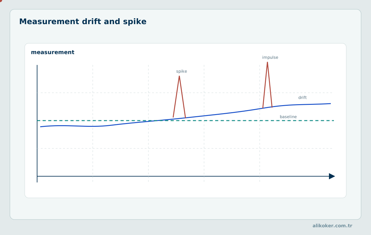
2.1. Observation equation

A simple model is yₜ = sₜ + nₜ + aₜ, separating signal, ordinary noise and contamination. For a nonlinear sensor, yₜ = h(xₜ) + vₜ + aₜ may be appropriate. Actual state changes must not be absorbed into the measurement-noise term, because that destroys the interpretation of later corrections.

2.2. Sampling and timestamps

Sampling frequency limits the shortest event that can be resolved. For irregular observations, an estimated slope is (xₜ − xₜ₋₁)/(tₜ − tₜ₋₁); replacing elapsed time with an index difference can create false spikes. Event time, arrival time and processing time should be distinguished.

2.3. Missingness, saturation and corrupted observations

A missing sample is not a numerical zero. Sensor saturation and digital clipping make the true magnitude beyond the range unobservable. A stuck sensor can appear statistically quiet despite being faulty. Missingness masks, units and calibration state should accompany the data.

2.4. Provenance and processing history

Original measurements, correction decisions and reconstructed values belong in separate fields. Algorithm, version, window and thresholds must remain identifiable. In forensic or safety-critical systems an estimate must never silently replace the original evidence.

2.5. Time alignment and data-quality checks

Identical nominal timestamps from two sensors do not guarantee physical synchronisation when their clocks differ. Clock drift, packet delay and batching can make a common event appear at different times. The clock source, sampling interval, allowed lateness and reordering policy must therefore be defined. Source-specific latency calibration or event-time windows may be preferable to direct timestamp equality.

Data-quality checks precede statistical anomaly decisions. Unexpected NaN/infinite values, physical range violations, duplicate sample identifiers, impossible time order and a stuck sensor require distinct quality flags. A numerically valid reading can still be physically impossible. These checks do not diagnose the event type; they prevent an anomaly model from learning from invalid input.

2.6. Propagation of measurement uncertainty

Derived quantities can amplify measurement uncertainty nonlinearly. For power P = V×I, a first-order variance approximation is Var(P) ≈ I²Var(V) + V²Var(I) + 2VI Cov(V,I). Ignoring covariance between voltage and current errors can give a misleading confidence interval. Likewise, a discrete derivative at constant sampling interval amplifies independent sample noise to a variance of about 2σ²/Δt².

Detection thresholds must therefore be dimensionally consistent. Retaining raw values, units, uncertainty and calibration status for every channel makes sensor-fusion decisions interpretable. When an extreme appears in a derived metric, measurement and alignment errors in its inputs should be checked first.

Unit 3: Probability and Statistical Decision Theory

Thresholding is not merely choosing a number; tail probability, false-alert risk and observation context must be interpreted together.

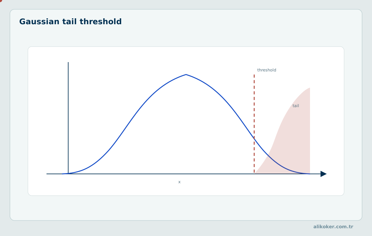
3.1. Distributions and tail probability

Mean μ and standard deviation σ summarise a distribution but do not define all its tail behaviour. P(X ≥ x) and P(X ≤ x) quantify rarity under a reference model. An assumed Gaussian model may produce misleading alerts for heavy-tailed financial returns or impulsive noise.

3.2. Hypotheses and decision cost

H₀ denotes data generated by the reference process; H₁ denotes departure from that process. False positives and false negatives need not have equal costs. Missing a flight-control fault may be more consequential than issuing an extra management warning. Threshold selection therefore combines statistics and operational loss.

3.3. Multiple testing

Testing one million true null hypotheses at α = 0.01 gives 10,000 expected false rejections regardless of independence, though dependence changes the distribution. False-discovery-rate procedures such as Benjamini–Hochberg address a different objective from family-wise error control.

3.4. Bayesian interpretation of rare events

For sensitivity 0.90, specificity 0.99 and event prevalence 0.001, the positive predictive value is 0.0009/(0.0009 + 0.00999) ≈ 0.0826. High sensitivity alone therefore does not establish a high probability that a flagged event is genuine.

3.5. Deriving a Bayesian decision threshold

For states H₀ (normal) and H₁ (event), the posterior is P(H₁|x) = p(x|H₁)P(H₁) / p(x). With false-alert cost C_FP, miss cost C_FN and zero correct-decision costs, an alert is optimal when P(H₁|x) > C_FP/(C_FP+C_FN). This does not assume independent consecutive observations or allow an arbitrary anomaly score to be treated as a probability; the posterior must be calibrated.

If missing an event costs 19 times as much as a false alert, the threshold becomes 1/(1+19) = 0.05. Rarity remains important because the prior is already incorporated in P(H₁|x). Review capacity and legal constraints can impose additional requirements on the decision rule.

3.6. Multiple testing and false discoveries

If 100 independent normal channels are each tested at α = 0.05, the probability of at least one false alert is 1 − (1 − 0.05)¹⁰⁰ ≈ 0.994. This calculation assumes independence; correlated channels require their joint dependence structure. Bonferroni bounds family-wise error, while the Benjamini–Hochberg procedure controls false discovery rate under its applicable assumptions.

A streaming detector tests related hypotheses repeatedly. Correcting simultaneous tests alone need not control false alarms over time. Repeated monitoring should be addressed with control charts, sequential testing or suitable online inference methods. Family-wise error, false discovery rate and false alerts per hour measure different operational quantities.

Sampling, probability models and hypothesis tests are developed in Probability and Statistics: Distributions, Sampling and Regression.

Unit 4: Time Series and Stochastic Processes

4.1. Dependence and stationarity

Treating correlated observations as independent can invalidate alert rates. Under weak stationarity, the mean is constant and covariance depends on lag rather than absolute time. Workday, seasonal and operating-mode patterns should be modelled before deviations are judged anomalous.

4.2. Forecasting models and residuals

An AR(p) model has xₜ = c + Σᵢφᵢxₜ₋ᵢ + εₜ. The residual εₜ = xₜ − x̂ₜ is the unexplained component. Testing residuals rather than raw observations can distinguish predictable seasonal peaks from unexpected events, but misspecified forecasts still mislead.

4.3. Regimes and change points

Distribution mean, variance, dependence or dynamic coefficients can change. After a change point, the earlier baseline may cease to apply. A short impulse and the first sample of a new regime can look identical; persistence, other channels or physical knowledge is needed to distinguish them.

4.4. Checking model adequacy

Residual mean, autocorrelation and variance stability should be checked. If a time-series model exhibits systematic errors during normal operation, large residuals cannot be trusted as anomaly evidence. Training and evaluation must respect time order.

4.5. Interpreting residuals after seasonal decomposition

A time series can be decomposed as yₜ = Tₜ + Sₜ + rₜ into trend, seasonal component and residual. A weekend sales increase can cross a fixed absolute threshold yet remain normal after conditioning on day of week. STL and related decompositions are meaningful only under suitable period, scale and robustness assumptions. Short series cannot support a reliable seasonal baseline; persistent regime shifts may instead be absorbed into the trend.

Residuals may be expected to resemble white noise, but this is a model-checking criterion rather than a guarantee. Residual autocorrelation invalidates independent-sample threshold calculations and can distort false-alert calibration. Raw observations, fitted expectations and residuals should be examined together.

4.6. Stochastic variation versus structural change

For an AR(1) process xₜ = φxₜ₋₁ + εₜ, the stationary model requires |φ| < 1. As φ approaches one, shocks persist longer; a sequence of elevated values does not by itself establish a new regime. Variation plausible under fixed φ may become a model mismatch when φ or innovation variance changes.

Before refitting a model, identify which mechanism may have changed: mean, variance, autocorrelation, seasonality or the input–output relation. No single threshold has equal sensitivity to all these alternatives.

The stochastic basis of arrival processes and system load is treated in Queueing Theory and Stochastic Processes.

Unit 5: Extrema, Spikes and Event Morphology

5.1. Local peak properties

A peak is characterised by prominence, width and rise/fall time in addition to height. Prominence reflects elevation relative to the surrounding baseline. Width depends on the selected level and must be expressed in time units when sampling frequency varies.

5.2. Differences and derivatives

The differences Δxₜ = xₜ − xₜ₋₁ and Δ²xₜ = xₜ − 2xₜ₋₁ + xₜ₋₂ reveal changes in slope and curvature. Differencing may amplify high-frequency noise. Thresholds should reflect both sensor resolution and physically plausible rates of change.

5.3. Short impulses and persistent steps

The value 50 in [10, 11, 10, 50, 10, 11] is a single-sample spike candidate; [10, 11, 10, 50, 51, 52] indicates a new level. A pointwise outlier test cannot separate them at onset; subsequent observations or a change detector are required.

5.4. Hysteresis and persistence

Choosing an entry threshold τₒₙ above the exit threshold τₒff can prevent alert chatter. Minimum duration, peak separation and re-trigger rules require event-specific calibration. Persistence rules must not suppress brief events that are physically meaningful.

5.5. Numerical comparison of a spike and a step

The series [10, 11, 10, 50, 10, 11] and [10, 11, 10, 50, 51, 52] share their first four samples. One reverts to baseline, while the other persists at a new level. A causal algorithm that has observed only the first four samples cannot know which future will occur. It can flag a departure, but classifying event type requires later observations or independent physical evidence.

5.6. Peak prominence and physical event duration

Peak height alone can miss short events under a changing baseline or broad oscillations. Prominence measures height relative to a surrounding contour level; together with width, rise time and fall time it distinguishes event shapes with similar amplitude. Minimum separation between peaks can incorrectly merge two genuine events. The neighbourhood window should reflect plausible physical event duration.

At a 1 kHz sampling rate, a three-sample impulse lasts approximately 3 ms, whereas 200 elevated samples last 200 ms. The two events can have identical peak height but different physical interpretations. Duration must therefore remain separate from amplitude in detection and classification.

5.7. Effect of differentiation on noise

If xₜ = sₜ + nₜ contains independent zero-mean measurement noise of variance σ², the noise contribution to the first difference nₜ − nₜ₋₁ has variance 2σ². When the difference is divided by sample interval Δt, the variance becomes 2σ²/Δt². Thus increasing sample rate does not justify proportionally reducing derivative thresholds at a fixed per-sample noise level.

Derivative detectors often use band limiting, local polynomial fitting or multiscale differences. Smoothing before differentiation can also spread short physical transitions. Detection delay, timing error and false-alert rate should be measured together.

Unit 6: Classical Outlier Tests

6.1. Standardised deviation

The score zᵢ = (xᵢ − μ)/σ measures standardised deviation. The common |zᵢ| > 3 rule is heuristic, not a universal error criterion. Outliers can shift both mean and standard deviation when these are estimated from contaminated data.

6.2. Interquartile range

IQR = Q₃ − Q₁, with conventional fences Q₁ − 1.5IQR and Q₃ + 1.5IQR. These fences flag candidates, not confirmed faulty measurements. Skewed and multimodal distributions can yield numerous flags for legitimate observations.

6.3. Assumptions of parametric tests

Grubbs and generalized ESD tests were developed for approximately Gaussian univariate data. Multiple contaminants and serial dependence can violate their assumptions. Test selection must consider sample size and any specified upper bound on the number of outliers.

6.4. Local and contextual baselines

A single global mean can misclassify valid readings when operating shifts or device types differ. Context groups should be defined without using future outcome labels, avoiding information leakage into the reference distribution.

6.5. Applicability of the generalized ESD test

The generalized ESD test addresses up to r outliers in an approximately normal univariate sample. At each step, the observation with the largest absolute standardised deviation is provisionally removed, and the mean and standard deviation are recomputed. The decision compares sequential statistics with critical values determined by the prespecified upper bound r and significance level α. Applying it directly to dependent time-series samples need not preserve nominal false-positive probability.

Trend, seasonality and distribution should be checked before selecting appropriate residuals for such a test. Detection does not authorise deletion: evidence that an extreme observation is erroneous must be assessed separately, as NIST also emphasises.

6.6. Local versus global thresholds

When observations come from multiple operating modes, a global mean can label the gap between valid modes as anomalous. Conversely, their pooled variance can hide genuine extremes. Local nearest-neighbour distance or density ratios may help in some geometries, but neighbourhood parameters become unstable in sparse data.

Threshold design should document distribution fit, sample count, contamination rate and minimum event duration. Convenient rules such as IQR fences do not automatically assign a tail probability to an observation.

Unit 7: Robust Statistics and Estimation

7.1. Median and median absolute deviation

Let m = median(x) and MAD = median(|xᵢ − m|). Under a roughly Gaussian distribution, σ̂ = 1.4826 MAD estimates scale. If MAD = 0, division must be avoided; a minimum scale based on instrument resolution or verified noise is preferable to an arbitrary dimensionless epsilon.

7.2. Hampel method

A local median mₜ and MAD scale yield a candidate rule |xₜ − mₜ| > kσ̂ₜ. Flagging and replacing are separate decisions. A centred window needs future samples; a causal window uses past data only and may behave differently at transitions.

7.3. Influence function and breakdown point

The influence function measures first-order sensitivity to infinitesimal contamination. The breakdown point is the limiting fraction of contamination that can drive an estimator arbitrarily far. The median’s high breakdown resistance does not guarantee correct event decisions under serial dependence or regime shifts.

7.4. Huber loss and robust regression

Huber loss equals 0.5r² for |r| ≤ δ and δ(|r| − 0.5δ) otherwise, limiting the influence of large residuals. The transition δ must be calibrated to residual units and scale. A robust training procedure must still preserve legitimate physical regime changes.

7.5. Worked example with median absolute deviation

For X = [10, 11, 10, 12, 150, 11, 10], the median is m = 11 and the absolute deviations are [1, 0, 1, 1, 139, 0, 1], giving MAD = 1. The robust scale estimate is σ̂ = 1.4826. For x = 150, the absolute robust standardised deviation is 139/1.4826 ≈ 93.75. The observation is clearly an outlier candidate; this does not establish whether it is faulty or physically genuine.

7.6. Robust location and scale estimation

For X = [10, 11, 10, 12, 150, 11, 10], the median is 11. Absolute deviations are [1,0,1,1,139,0,1], giving MAD = 1 and a Gaussian-calibrated robust scale of approximately 1.4826. The deviation of 150 is about 93.8 robust scale units. If MAD were zero, this statistic would be undefined; measurement resolution and a minimum noise floor must be specified beforehand.

A moving-window median can itself move as contamination grows. When a genuine new level appears, a centred reference window can suppress the transition. Outlier flagging and acceptance of a new operating regime therefore require distinct policies.

7.7. Limiting influence in robust regression

For squared loss L(r) = 0.5r², the derivative equals r, so a large erroneous observation can exert unbounded influence on parameter updates. Huber loss limits the derivative to δ×sign(r) when |r| > δ. This reduces influence but does not prove that the observation has been correctly classified as corruption. Residual units and δ must agree.

RANSAC instead builds candidate models from random subsets and counts consistent observations. Success depends on inlier proportion, model identifiability, sampling and consensus threshold. Reproducibility requires recording the random seed and iteration limit.

Statistical prerequisites for robust estimation are found in Probability and Statistics: Distributions, Sampling and Regression.

Unit 8: Multivariate Anomalies and Extreme Values

8.1. Mahalanobis distance

The statistic d² = (x − μ)ᵀ Σ⁻¹(x − μ) incorporates correlations. Two sensor readings that are individually ordinary may form an unlikely combination. Singular or ill-conditioned covariance matrices require regularisation or an appropriate linear solver rather than naïve inversion.

8.2. Robust covariance

Sample covariance can be distorted by contamination. Methods such as Minimum Covariance Determinant provide more resistant location and covariance estimates. When dimension approaches sample count, dimensionality reduction or regularisation may also be necessary.

8.3. Extreme value theory

Block maxima can be modelled with the generalised extreme value (GEV) family; sufficiently high exceedances may be approximated by a generalised Pareto distribution under suitable conditions. A low threshold weakens the asymptotic approximation, while a high threshold leaves too few samples.

8.4. Dependent extreme events

Consecutive extremes need not be independent events. Network bursts, seismic aftershocks or volatility clustering affect exceedance counts and uncertainty intervals. Event-level analysis should estimate cluster onset and duration separately.

8.5. Two-dimensional distance example

Consider μ = [0, 0], Σ = diag(1, 4) and x = [3, 4] for independent coordinates. The squared Mahalanobis distance is d² = 3²/1 + 4²/4 = 13. Under a known correct bivariate Gaussian model, the 99% chi-square threshold with two degrees of freedom is about 9.21, so this observation exceeds it. Estimating covariance from the tested sample changes the inference and requires additional care.

8.6. Geometric anomalies in correlated channels

Individually ordinary sensor readings need not form an ordinary joint observation. Two temperature sensors may normally agree, so (20,20) and (30,30) are plausible while (20,30) is inconsistent despite each component falling within its marginal range. Mahalanobis distance uses covariance-defined elliptical geometry to highlight this discrepancy. A single covariance matrix is inadequate when cross-sensor relationships depend on operating mode.

Covariance inversion becomes unstable with many features and few samples. Shrinkage covariance, dimension reduction and numerical linear solves are preferable. A chi-square threshold requires checking the distributional model and how its parameters were estimated.

8.7. Dependence and clustering of extremes

Extreme-value modelling must account for dependent consecutive exceedances. Heavy rainfall, volatility clustering or network bursts may produce many elevated samples from one episode. Declustering can treat correlated samples as one event, while persistent inter-cluster dependence still affects uncertainty estimates.

Block maxima and peaks-over-threshold have different bias–variance trade-offs. Too low a threshold weakens the tail approximation; too high a threshold leaves insufficient observations. A modelled return level does not predict the exact time of a future extreme event.

Unit 9: Sequential Statistical Detection

9.1. Control charts

A Shewhart chart responds to large individual departures; EWMA and CUSUM target smaller sustained shifts with different detection delays. Control limits encode a probability model and expected false-alert behaviour. An out-of-control sample should not be automatically removed as a measurement error.

9.2. CUSUM calculation

A one-sided standardised CUSUM can be written Cₜ = max(0, Cₜ₋₁ + zₜ − κ), with an alert when Cₜ > h. The allowance κ relates to the target shift, while h trades false alerts against detection delay. Persistent small deviations can accumulate despite never crossing a pointwise threshold.

9.3. Sequential likelihood ratios

SPRT accumulates log(P(x|H₁)/P(x|H₀)) as samples arrive. Its interpretation depends on hypotheses and distributional assumptions. Generalised likelihood ratios also estimate unknown change parameters, typically increasing model and computational complexity.

9.4. Alert rate and detection delay

Average run length (ARL) measures expected samples until a signal, not necessarily elapsed-time delay. Sampling frequency, reset policy and dependence structure must be controlled in comparisons.

9.5. Sequential CUSUM calculation

Let κ = 0.5, h = 1.5, C₀ = 0 and z = [0.1, 0.2, 1.2, 1.1, 1.1]. Applying Cₜ = max(0, Cₜ₋₁ + zₜ − κ) gives 0, 0, 0.7, 1.3 and 1.9. The first alarm occurs at sample five, whereas a pointwise |zₜ| > 3 rule does not alarm. These illustrative parameters do not guarantee a specified false-alert rate.

9.6. CUSUM threshold, average run length and sample count

CUSUM accumulates small shifts, making false-alert behaviour a sequential rather than one-shot property. In Cₜ = max(0,Cₜ₋₁+zₜ−κ), allowance κ reflects the shift of interest while threshold h trades delay against false alerts. ARL₀ is the expected run length under the reference process; ARL₁ characterises run length after a change. The same run length can represent very different wall-clock delays at different sample rates.

Reset behaviour, hold-off intervals and duplicate-event policies need explicit specification. Parameters should be checked against false alerts during normal periods as well as detection speed after a simulated shift.

9.7. Conditional likelihood and independence assumptions

The recursive log-likelihood ratio log Λₜ = log Λₜ₋₁ + log[p(xₜ|H₁)/p(xₜ|H₀)] is appropriate only when its likelihood model captures the observation process. For dependent samples, conditional terms p(xₜ|x₁:ₜ₋₁,H) are needed; treating correlated samples as independent can double-count evidence. If onset is unknown, candidate change points must also be considered.

Generalised likelihood-ratio tests estimate unknown parameters from current data, offering flexibility at greater computational and calibration cost. A practical architecture can use a constant-cost control statistic first and a more expensive test on selected events.

The probabilistic foundations of sequential testing connect to Probability and Statistics: Distributions, Sampling and Regression.

Unit 10: Change Points and Distribution Drift

Persistent breaks in mean, variance or shape are often more important than isolated outliers. A segmented view makes the change point interpretable.

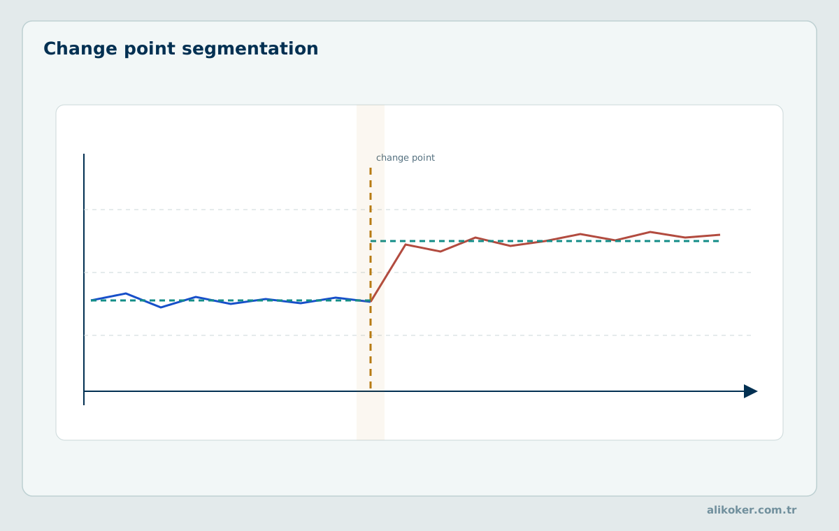
10.1. Multiple change points

For changes at τ₁, τ₂, …, one may minimise J = Σⱼ C(segmentⱼ) + βK, balancing segment fit and number of changes. PELT can exploit pruning under appropriate cost conditions, but is not guaranteed linear time for every series.

10.2. Bayesian online change-point detection

A probability distribution over run length—the time elapsed since the most recent change—can be updated with each observation. The hazard prior, predictive likelihood and approximation strategy directly affect online change probabilities.

10.3. Adaptive windows and concept drift

ADWIN uses adaptively sized windows to detect changes. Concept drift, covariate shift and model-performance degradation are not synonymous: input distribution can move while the conditional target relation remains stable. The distinction informs retraining decisions.

10.4. Safe baseline adaptation

Immediately incorporating suspicious samples into the baseline may normalise a genuine anomaly. Updates can be delayed, bounded or restricted to verified normal periods. Conversely, refusing to recognise a legitimate new regime causes persistent alerts; an explicit policy must balance these failures.

10.5. Choosing penalties for multiple change points

Segmenting a series into K+1 parts with J = Σ C(segmentⱼ) + βK balances fit against unnecessary change points. A small β creates many noise-driven splits; a large β merges short genuine regimes. The selected cost—mean shift, variance shift or distributional change—can yield different segmentations on the same data.

If variance doubles while the mean remains constant, a cost focused only on within-segment mean squared error may miss the change. A Gaussian likelihood with segment-specific variance may be more suitable. PELT pruning depends on cost assumptions and does not guarantee linear complexity on every dataset.

10.6. Taxonomy of distribution shift

Covariate shift changes P(X) while P(Y|X) remains stable. Concept drift changes the conditional decision relation P(Y|X); label shift may alter P(Y). Retraining without identifying the mechanism can absorb a new regime while erasing previous safety boundaries.

Systems with delayed labels cannot measure real-time classification accuracy immediately. Distributional monitoring, calibration monitoring and interpretable operational indicators should be reported separately. Later event labels must be checked for selection bias before entering the next training set.

Unit 11: Anomaly Scores, Red Flags and Alert Management

A red flag is a decision summary built from several weak indicators. A high score warrants review; it is not a verdict on its own.

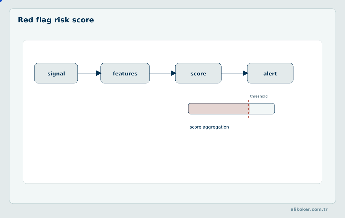
11.1. Anomalies versus red flags

Anomaly scores quantify deviation from a baseline. A red flag is a statistical, rule-based or contextual indicator that may justify review. Not every outlier is risky; a suspicious authorisation change may raise a red flag without being a numerical outlier.

11.2. Score calibration and alert thresholds

Raw scores from different detectors are not directly comparable. Thresholds should reflect event prevalence, analyst capacity and the cost of missed incidents. Sensitivity, specificity and precision require separate reporting. A fixed daily alert quota cannot guarantee safety without evaluating missed-event risk.

11.3. Alert grouping and review

Hundreds of alerts from one root cause can be grouped into a case. Grouping uses source, time, relationships and physical context, but must not merge distinct incidents and obscure evidence. Confirmed and dismissed alerts should be examined for selection bias before becoming training labels.

11.4. Decision cost and human oversight

A flagged indicator is not proof of crime, fault or intrusion. Financial-crime, security and forensic workflows should distinguish observations, computed indicators, thresholds, independent evidence and human review. Alert fatigue and explainability are operational quality concerns.

11.5. Positive predictive value for rare alerts

At 0.1% event prevalence in 100,000 observations, one expects 100 actual events. A system with 90% sensitivity detects about 90 of them. At 99% specificity, roughly 999 of the 99,900 normal observations are false positives. PPV = 90/(90 + 999) ≈ 8.26%. These expectations assume fixed test properties; correlated event windows additionally require event-based assessment.

11.6. Separating risk indicators from evidence

A red flag is a signal that changes review priority; it does not establish the cause or legal status of unusual behaviour. Many transfers to one account in a short period may arise in legitimate collections or suspicious patterns. Amounts, customer profile, linked parties, timing and stated purpose need to be considered together. Indicators can originate from rules, statistical deviations or both.

A weighted score is not automatically a calibrated probability. Its coefficients depend on label quality, event prevalence and review cost. An alert decision and a verified finding should be represented as different record types.

11.7. Review capacity and threshold optimisation

If N candidates are scored per hour, the expected review load at threshold τ is N×P(score≥τ). Analyst capacity B constrains that load, but retaining only the top B scores does not prove that missed lower-scoring events are acceptable. Thresholds should reflect false-alert, missed-event and review costs.

With a hypothetical 10,000 transactions/day, 0.1% prevalence, 90% sensitivity and 99% specificity, about 9 true alerts and 100 false alerts are expected; positive predictive value is roughly 8.3%. These are illustrative assumptions, not institutional measurements. Grouping alerts may reduce workload, but its event-level false-negative effect must still be assessed.

The decision cost of an alert threshold relates to Decision Support Systems: Decision Analytics, Optimization, Uncertainty, and Decision Intelligence; its security-operations consequences relate to Cybersecurity Engineering.

Unit 12: Linear Digital Filters

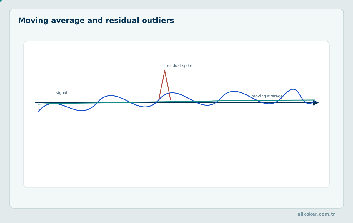
In practice the goal is often not to suppress the signal but to separate slow trend and inspect the residual structure. A moving average makes that decomposition visible.

12.1. Convolution and frequency response

For a linear time-invariant system, y[n] = Σₖ h[k]x[n−k], where h is the impulse response. Frequency response determines attenuated components. If the rejected band contains real event energy, a smoother output is obtained without any guarantee of correctness.

12.2. FIR and IIR structures

Finite impulse response (FIR) filters can provide linear phase through suitable coefficient symmetry. Infinite impulse response (IIR) filters may achieve comparable selectivity with lower order, at the cost of additional phase and stability considerations.

12.3. Classical filter families

Butterworth, Chebyshev, elliptic and Bessel designs prioritise passband smoothness, selectivity or phase/group-delay behaviour differently. Sampling rate, tolerances, filter order, fixed-point precision and event timing all affect selection.

12.4. Causality and forward-backward application

A causal filter uses present and past observations only. Forward-backward filtering may cancel phase shift but requires future samples and cannot run directly within a strict zero-lookahead stream. Filter-induced delay must be part of the real-time contract.

12.5. Latency–selectivity trade-off in FIR and IIR design

A causal M-tap FIR filter uses yₙ = Σₖ₌₀ᴹ⁻¹ bₖxₙ₋ₖ and typically requires O(M) multiply-add operations per sample. Symmetric linear-phase coefficients can introduce group delay (M−1)/2 samples. For 101 taps at 1 kHz, this is about 50 ms, which may be unacceptable for a detector requiring a response within a few milliseconds.

An IIR design may achieve comparable frequency selectivity with fewer coefficients, but pole locations, numerical quantisation and phase response become important. A sharper cutoff is not automatically superior; it trades amplitude distortion and transition width against latency and numerical behaviour.

12.6. Separating filtering from event detection

A low-pass filter attenuates high-frequency noise but can also attenuate a genuine impulse in the same band. Pre-detection filtering and post-event display filtering can therefore use separate paths. Running an energy/peak detector on raw samples alongside a slow-regime detector on filtered samples may reduce information loss.

Forward–backward zero-phase filtering uses future observations and is appropriate for offline reanalysis, not as a direct equivalent of strict causal online processing. Timing and phase of a filtered output must not be confused with event time in the raw signal.

System-theoretic foundations of convolution and frequency response are covered in Signals and Systems.

Unit 13: Nonlinear and Adaptive Filters

13.1. Median and Hampel filters

A median filter returns the middle order statistic of a window and can suppress isolated impulses, but may erase genuine short peaks. Hampel filtering is more selective when only flagged samples are replaced. Both depend on window length and boundary handling.

13.2. Local polynomial and total variation methods

Savitzky–Golay filtering fits a local polynomial and can retain peak shape better than a moving average for suitable parameters. Total variation denoising penalises the sum of |xₜ − xₜ₋₁| to favour piecewise regularity. Excessive regularisation can erase small real changes.

13.3. Adaptive LMS and RLS

LMS adapts weights from instantaneous squared-error gradients; NLMS scales its step using input energy. RLS can adapt faster with an appropriate forgetting factor but uses more computation and state. The noise reference must actually represent the unwanted component.

13.4. Wiener estimation

Wiener filtering targets minimum mean squared error using second-order statistics. Estimated signal and noise spectra are themselves uncertain. Reusing stale statistics across a regime change can suppress the very event being sought.

13.5. Local smoothing and edge preservation

Savitzky–Golay fits a low-degree polynomial to a local window to estimate the centre value or derivatives. With a suitable degree and sufficient samples, it can preserve some peak shapes better than a moving average, but may overshoot near sharp steps. A median filter removes isolated impulses while potentially deforming genuine transients extending over several samples. Total-variation regularisation favours piecewise-smooth or piecewise-constant structure.

The choice depends on the property to preserve: peak height, transition time, band energy, derivative or baseline. A smoother curve is not necessarily more accurate under all those criteria. Detection and display pipelines may use different representations.

13.6. Reference-signal requirements for adaptive filtering

A standard LMS update is wₙ₊₁ = wₙ + μeₙxₙ, with sign and scaling determined by the error and objective definitions. Convergence depends on choosing step size μ consistently with input energy and eigenvalue spread. NLMS normalises by input energy and may adapt more reliably across amplitude ranges. RLS can track changes faster but incurs matrix-update cost and requires careful forgetting-factor selection.

An adaptive noise-cancellation reference may contain correlated target information; the filter can then suppress the event itself. Reference-to-target dependence must be examined, especially when multiple microphones capture the same acoustic source.

Unit 14: Time–Frequency and Multiscale Analysis

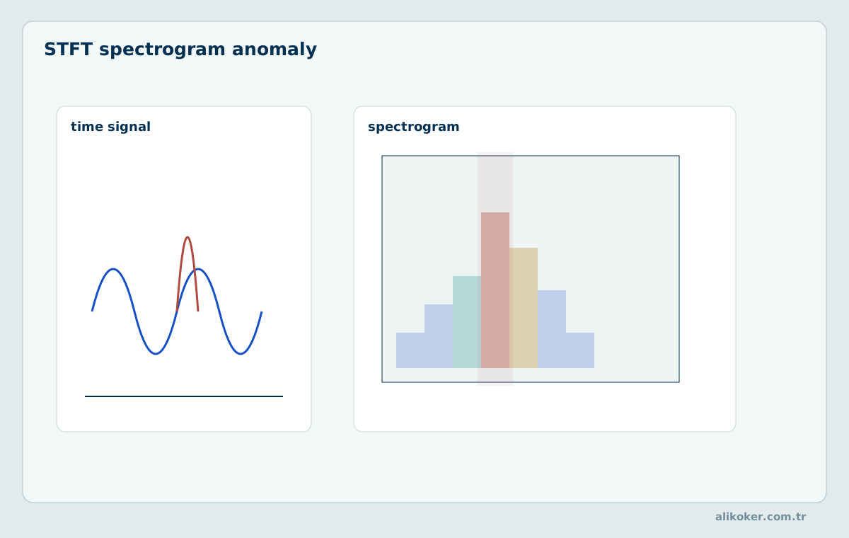
Short transient events may remain ambiguous in the raw series. A time–frequency representation reveals when and in which band the event occurs.

14.1. Short-time Fourier transform

The short-time Fourier transform analyses frequency content in local windows. Short windows improve timing resolution; long windows improve frequency resolution. Window leakage, scaling and overlap must be specified when timing transients.

14.2. Wavelet transform

Wavelet transforms produce coefficients localised at multiple time and frequency scales. Short impulses may stand out at fine scales, while slow changes appear at coarse scales. Wavelet family, boundary extension and decomposition level materially affect results.

14.3. Thresholding and sparse representations

Soft thresholding wavelet coefficients can reduce noise: ŵ = sign(w)·max(|w| − λ, 0). An excessive λ removes legitimate transients. Sparse representation by itself does not guarantee that low-energy event details are preserved.

14.4. Spectral kurtosis and mode decomposition

Spectral kurtosis can reveal bands with strongly impulsive energy but is not a fault diagnosis by itself. Rotating machinery, underwater acoustics and seismology require physical context. EMD and VMD decompositions should be checked for mode mixing and parameter sensitivity.

14.5. Soft-thresholding wavelet coefficients

With coefficients w = [−5, 1, 3] and threshold λ = 2, soft thresholding sign(w)·max(|w| − λ, 0) produces [−3, 0, 1]. Removing small coefficients may suppress noise, but it also removes information when those coefficients belong to real events. Threshold selection requires validation against noise and relevant event signatures.

14.6. Time–frequency resolution in practice

For an N-sample STFT window at sampling rate fₛ, the nominal bin spacing is Δf = fₛ/N. At 8 kHz with N = 256, spacing is 31.25 Hz; with 1024 samples it is 7.8125 Hz, while window duration grows from 32 ms to 128 ms. Bin spacing is not identical to practical resolution of two close tones, which also depends on the window and spectral leakage.

A shorter window may localise a brief impulse in time; a longer window may be needed for narrowband harmonic changes. Multiresolution methods address this trade-off through different scales. Zero-padding interpolates the displayed spectrum but does not inherently improve physical frequency resolution.

14.7. Bias and event loss in wavelet thresholding

In an orthogonal wavelet representation, coefficients cⱼₖ contain both noise and legitimate weak details. Hard thresholding zeros coefficients with |c| ≤ λ; soft thresholding uses sign(c)×max(|c|−λ,0). Soft thresholding avoids a hard discontinuity but shrinks large coefficients by λ and introduces bias. Wavelet support also affects temporal spreading of short events.

Noise-scale estimation can itself be distorted by impulsive events. A denoised reconstruction should be evaluated for energy, onset timing and transient amplitude before it is judged successful.

Frequency resolution and multichannel signal concepts connect to Signals and Systems.

Unit 15: Harmonics, Resonance and Waveform Distortion

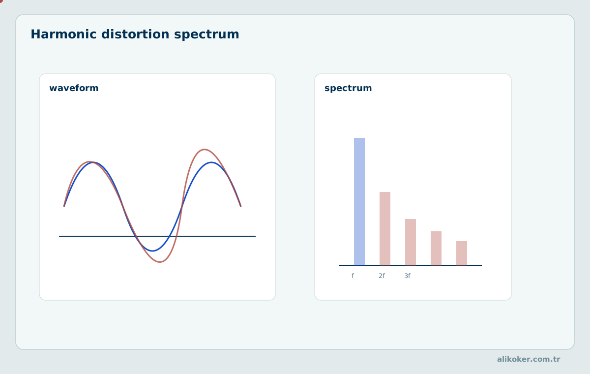
Periodic distortions can be tracked as harmonics added to the fundamental component. Both waveform and spectrum are needed for proper interpretation.

15.1. Fundamental frequency and harmonics

A periodic waveform may contain a fundamental f₀ and harmonics nf₀. Harmonics are normal components of speech and music. In power systems nonlinear loads may inject current harmonics that affect network voltage and equipment, but the objective is not to remove every harmonic component.

15.2. Total harmonic distortion

For voltage, THDᵥ = √(Σₙ≥₂ Vₙ²)/V₁ is computed over specified harmonic components and RMS definitions; a corresponding current metric exists. IEEE 519-2022 addresses steady-state harmonic goals at the point of common coupling, not unrestricted assessment of every transient.

15.3. Interharmonics, transients and resonance

Components not at integer multiples of the fundamental are interharmonics. Short switching events can produce broadband transients. At resonance, the transfer function amplifies selected frequencies. A fixed notch filter does not, by itself, remedy these physical causes.

15.4. Distinct acoustic and electrical decisions

Reducing upper harmonics in audio can distort timbre; in an electrical installation specified harmonic limits may be essential to power quality. The same Fourier coefficients support different engineering decisions. Measurement point and operating objective must be stated before selecting any correction.

15.5. Calculation of total harmonic distortion

For an illustrative voltage measurement, take V₁ = 230 V RMS, V₃ = 11.5 V and V₅ = 6.9 V. Considering only these two higher harmonics yields THDᵥ = √(11.5² + 6.9²)/230 ≈ 0.0583, or 5.83%. This calculation alone cannot establish violation of a power-quality standard; measurement point, other harmonics and applicable limits matter.

15.6. Physical interpretation of harmonic power

For RMS harmonic magnitudes V₁,V₂,…, a common voltage total harmonic distortion measure is THDᵥ = √(Σₕ₌₂ᴴ Vₕ²)/V₁. Values are not comparable without stating the measurement bandwidth, included harmonic orders and fundamental-frequency estimator. Interharmonics are not integer multiples of the fundamental and should not be combined indiscriminately under the same convention. Operating conditions and measurement location matter.

In power systems, acceptability of distortion depends on the standard's definitions and point of measurement. Elevated harmonic content alone does not establish equipment failure. In acoustic signals, higher harmonics are often normal components of timbre.

15.7. Resonance, low-frequency oscillation and event detection

Resonance peak width and centre frequency relate to damping. In rotating machinery, a rise near a natural frequency may reflect forced response during speed changes; a newly persistent narrowband component can instead prompt investigation of bearings, connections or control loops. Speed-synchronised spectra, envelope analysis and operating history support the distinction.

Strong energy in a short-time spectrum does not by itself distinguish a sustained harmonic from a window-smeared transient. Time–frequency persistence, harmonic ratios and phase behaviour should be considered together.

Harmonics in power converters relate to Power Electronics; their role in acoustic timbre relates to Audio Processing and Forensic Audio Engineering.

Unit 16: Missing-Data Imputation and Signal Reconstruction

16.1. Conditions for valid reconstruction

Samples should not be overwritten until measurement error has been sufficiently established. Short gaps may be approximated by interpolation, but this does not recover the unknowable original value. Reconstruction uses only information supported by the model and neighbouring observations.

16.2. Interpolation and local replacement

Linear interpolation joins valid neighbouring points with a straight line. Cubic splines produce smooth derivatives; PCHIP is more shape-preserving but cannot infer an unknown true discontinuity. Median replacement is appropriate only for confirmed short measurement impulses.

16.3. Model-based imputation

ARIMA, Kalman prediction or Gaussian-process regression can supply a predictive distribution. Uncertainty should accompany the point estimate where possible. Longer gaps should normally increase uncertainty rather than produce unjustifiably narrow intervals.

16.4. Forensic and safety-critical data

The original recording, damage mask, reconstruction method and derived result remain distinct. Reconstructed audio or imagery may support analysis but must be identified as an estimate rather than original content. Reproducible processing parameters and unchanged evidence should be retained.

16.5. Mechanisms of missing data

Missingness can influence conclusions. Missing completely at random (MCAR), missing at random conditional on observed variables (MAR), and missing not at random (MNAR) require different assumptions. If a sensor disconnects only at extreme temperatures, interpolating across the gap can systematically erase the very extremes of interest. Reconstructed values must retain an uncertainty or missingness indicator.

Linear interpolation over long gaps does not recover physical dynamics; it expresses a smoothness assumption. Acceptability should be assessed relative to the system's characteristic time scale and the duration of missing data.

16.6. Error budget for correction methods

Keep the original observation yₜ, acceptance decision aₜ and corrected estimate x̂ₜ separate. Correction may be justified when physical measurement failure is independently established; otherwise retain an uncertainty flag. Performance is evaluated against validated reference data using numerical error, timing shift and preservation of physical quantities, not how smooth the resulting plot looks.

A few onset samples can be scientifically or legally decisive in seismic, acoustic or forensic material. Every reconstructed interval must be identifiable. The original record should not be overwritten irreversibly.

Image restoration and the forensic status of reconstructed detail are considered in Image Processing and Computer Vision Engineering.

Unit 17: State Space Models and Observers

17.1. Latent state model

A discrete linear system is xₖ = Fxₖ₋₁ + Buₖ + wₖ and zₖ = Hxₖ + vₖ. The latent state x differs from known input u, process uncertainty w and measurement uncertainty v. A physical fault may change dynamics, whereas a sensor fault affects observations.

17.2. Observability

The ability to infer hidden states depends on observability. For a linear system, the observability matrix O = [H; HF; …; HFⁿ⁻¹] having full column rank provides a theoretical condition. Numerical conditioning still matters.

17.3. Residual-based fault detection

The innovation rₖ = zₖ − Hx̂ₖ⁻ measures disagreement between observation and prediction. A large residual is not proof of sensor failure: a real manoeuvre, delayed packet, incorrect parameter or wrong unit can cause the same symptom.

17.4. Luenberger observer

An observer uses a gain L to correct predictions from measurement residuals; index alignment must match the chosen observer convention. The gain governs the stability and response of estimation-error dynamics.

17.5. Limits of observability and identifiability

For linear xₖ₊₁ = Fxₖ + Buₖ and yₖ = Hxₖ, the observability matrix is O = [H; HF; HF²; …; HFⁿ⁻¹]. With state dimension n, rank(O) < n means some state components cannot be distinguished from the outputs alone. A Kalman filter may still produce numbers for those components without gaining valid information. Sensor placement, sampling and operating regime affect practical observability.

If two faults produce indistinguishable residuals, detection may be possible while fault isolation is not. The distinction between detection and diagnosis depends on structural identifiability. Multisensor design must also account for common-mode failures.

17.6. Observer residual and model mismatch

A Luenberger observer may update through x̂ₖ₊₁ = Fx̂ₖ + Buₖ + L(yₖ − Hx̂ₖ). Its residual rₖ = yₖ − Hx̂ₖ can increase because of unknown inputs, parameter mismatch, sensor errors or genuine dynamic events. A large residual is therefore not equivalent to a sensor failure. Error-dynamics eigenvalues and noise assumptions affect detection delay.

Residual signatures may be designed to respond differently to faults, but diagnosis requires those signatures to be identifiable. Thresholds learned in one regime must be checked across all intended operating modes.

State space, observability and observer design share their mathematical basis with Automatic Control: Theory, Analysis, Design, and Practice.

Unit 18: Kalman Filtering and Measurement Consistency

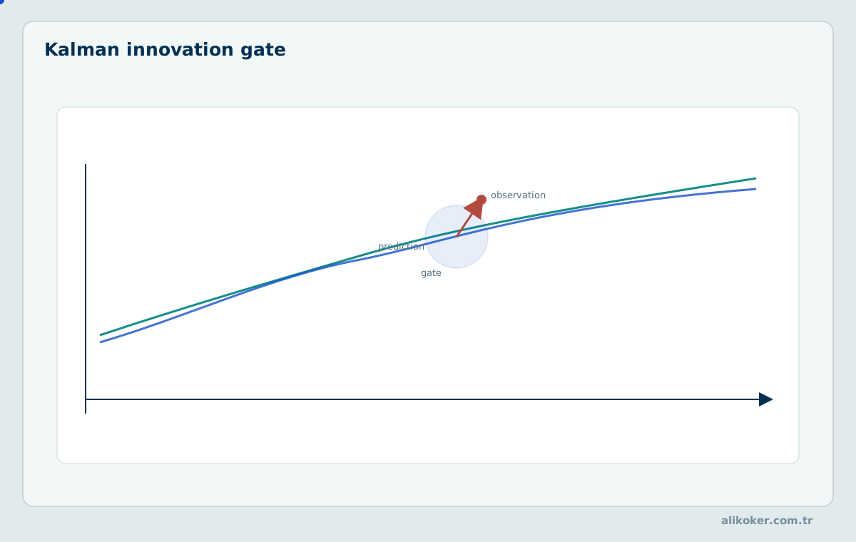
The discrepancy between prediction and observation is not an absolute error alone; it is evaluated under uncertainty. Innovation gating is a core mechanism for rejecting inconsistent measurements.

18.1. Prediction and update

Prediction: x̂ₖ⁻ = F x̂ₖ₋₁ + Buₖ; Pₖ⁻ = FPₖ₋₁Fᵀ + Q. Innovation: νₖ = zₖ − Hx̂ₖ⁻; covariance: Sₖ = HPₖ⁻Hᵀ + R. Gain Kₖ = Pₖ⁻HᵀSₖ⁻¹; update x̂ₖ = x̂ₖ⁻ + Kₖνₖ. Linear solves are preferable to explicitly forming a matrix inverse.

18.2. Covariance and numerical reliability

Q expresses process-model uncertainty and R measurement uncertainty. An underspecified Q can cause sluggish tracking of genuine manoeuvres; a large R downweights observations. The Joseph form P = (I−KH)P⁻(I−KH)ᵀ + KRKᵀ helps retain favourable covariance properties numerically.

18.3. Normalised innovation squared

NIS = νᵀS⁻¹ν scales the innovation by its covariance. Under a correctly specified linear Gaussian model it can be compared with χ²(m), where m is the measurement dimension. A high NIS flags model–measurement inconsistency; a genuine manoeuvre or regime change must be considered before rejecting the observation.

18.4. Prediction under missing observations

When a valid measurement is unavailable, prediction and covariance propagation may continue without an update. Growing uncertainty should remain visible. Automatically rejecting a channel indefinitely can prevent convergence to a new true state; re-admission conditions are required.

18.5. Scalar Kalman update

Let prior mean x̂⁻ = 20, prior variance P⁻ = 4, observation z = 24, observation variance R = 9, and H = 1. Innovation ν = 4 and S = 13 give gain K = 4/13 ≈ 0.3077. Posterior mean is x̂ = 20 + (4/13)×4 ≈ 21.23 and variance is P = 36/13 ≈ 2.77. NIS = 16/13 ≈ 1.23. Observation disagreement must be evaluated relative to uncertainty.

18.6. Numerical example of Kalman gain

For a scalar prediction x̂⁻ = 20 with variance P⁻ = 4, measurement z = 26 and measurement variance R = 5, the gain is K = P⁻/(P⁻+R) = 4/9 ≈ 0.4444. The updated state is x̂ = 20 + (4/9)×(26−20) ≈ 22.6667 and posterior variance is P = (1−4/9)×4 = 20/9 ≈ 2.2222. Model and measurement are weighted by uncertainty rather than replacing the state with 26.

Innovation ν = 6 and its variance S = 9 give NIS = ν²/S = 36/9 = 4. Under a correctly specified scalar Gaussian measurement model, this can be assessed against chi-square with one degree of freedom, but a single elevated NIS does not identify the fault cause.

18.7. Numerical preservation of covariance

The Joseph covariance update is P⁺ = (I−KH)P⁻(I−KH)ᵀ + KRKᵀ. Under finite precision, using only P⁺ = (I−KH)P⁻ can amplify asymmetry and loss of positive semidefiniteness. Cholesky/QR-based linear solves or square-root filtering can avoid explicit inversion. A non-positive-definite innovation covariance S requires investigation of the model, R assumptions and numerical implementation.

Changing Q or R merely to make a graph visually smooth does not ensure consistent estimation. Innovation mean, autocorrelation and NIS coverage should be checked across operating regimes.

Estimation constraints in feedback and control systems are discussed in Automatic Control: Theory, Analysis, Design, and Practice.

Unit 19: Nonlinear Kalman Filter Families

19.1. Extended Kalman filter

For nonlinear transitions xₖ = f(xₖ₋₁,uₖ)+wₖ and observations zₖ = h(xₖ)+vₖ, EKF uses local Jacobians. Strong nonlinearity or poor initialisation can invalidate local approximation. Jacobian and covariance dimensions must remain consistent.

19.2. Unscented Kalman filter

UKF propagates selected sigma points through nonlinear functions to approximate moments without Jacobians. It does not generally represent a multimodal posterior exactly. Sigma-point weights and covariance positivity require care.

19.3. Cubature and square-root methods

Cubature Kalman filters approximate Gaussian integrals using selected integration points. Square-root forms propagate a covariance factor and may improve numerical stability. Selection depends on state dimension, uncertainty structure and compute budget.

19.4. Limits of adaptation

Online noise-covariance adaptation can improve fit, but adapting aggressively to suspect observations can conceal anomalies. Updates require physical bounds and independent consistency checks.

19.5. Approximation differences between EKF and UKF

For nonlinear measurement z = h(x) + v, EKF linearises h around the estimate using Jacobian H = ∂h/∂x. Strong curvature, large initial error or derivative discontinuities can invalidate the local approximation. UKF propagates selected sigma points through h to approximate transformed means and covariances; it avoids Jacobians but depends on point weights, scaling parameters and state dimension.

A more elaborate method is not automatically more accurate. EKF may be sufficient for smooth near-linear dynamics, while a high state dimension or unsuitable sigma-point scaling can increase UKF cost and numerical risk. Incorrect system dynamics affect both approaches.

19.6. Consistency tests in nonlinear estimation

For nonlinear estimators, innovations need not remain exactly Gaussian. A theoretical chi-square NIS threshold can then become only an approximate consistency check; empirical calibration may be required under strong nonlinearity and poor initial conditions. When simulation provides ground truth, NEES = (x−x̂)ᵀP⁻¹(x−x̂) can be evaluated. NEES cannot be computed directly in production without knowing the actual state x.

Experiments should use comparable initial covariance, observation model, sampling and compute budgets. Reporting mean position error alone does not establish consistency or tail-error behaviour.

Unit 20: Robust and Multiple-Model State Estimation

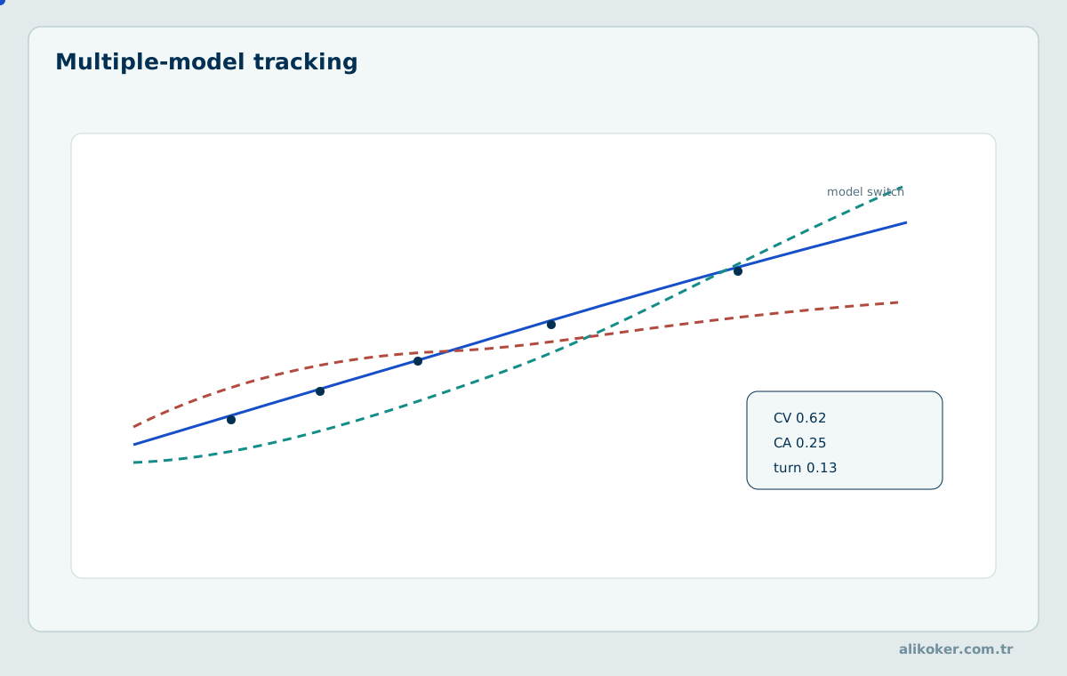
Target dynamics are rarely fixed. Reweighting multiple motion models is more reliable than a single-model assumption under abrupt maneuvers and regime changes.

20.1. Innovation gating and robust loss

A measurement with excessive NIS may be downweighted or temporarily rejected. Residual magnitude alone can also reject a real rapid manoeuvre. Huber loss and heavy-tailed Student-t measurement models provide alternatives for contaminated observations.

20.2. H-infinity and strong tracking

H-infinity filtering targets bounded worst-case sensitivity to model uncertainty; this differs from Kalman optimality under a probabilistic model. Strong-tracking methods may follow abrupt dynamics faster, but can amplify measurement noise.

20.3. Interacting multiple models

Interacting multiple-model filters maintain probabilities over alternative dynamics. A tracked target alternating between constant-velocity, acceleration and manoeuvre modes may not be well represented by a single model. Transition probabilities must reflect the application.

20.4. Particle filtering

Particle filters represent posterior distributions by weighted samples. They support nonlinear and non-Gaussian cases, but particle count, resampling and weight degeneracy govern cost. High-dimensional states can require prohibitively many particles.

20.5. Gating, robust estimation and abrupt manoeuvres

NIS gating can classify a measurement as statistically surprising relative to the current estimate. However, an aircraft manoeuvre can generate large innovations when the filter assumes constant velocity. Rejecting every such measurement may cause loss of track. Alternatives include conditional inflation of measurement covariance, robust loss, adaptation of process uncertainty or switching to a manoeuvre model.

None is universally correct. Increasing R weakens measurement influence, whereas increasing Q raises model uncertainty and alters responsiveness to dynamic change. If sensor error, model error and physical manoeuvre cannot be distinguished, the ambiguity must remain explicit.

20.6. Interacting multiple models and particle methods

IMM updates several motion models and their probabilities jointly. Combining constant-velocity, constant-acceleration and turning models can reduce the bias of a single model during manoeuvres. Poor transition probabilities, however, prevent the model set from representing real regimes. More models also increase compute and calibration burden.

A particle filter can represent non-Gaussian or multimodal state distributions, but weight concentration causes particle degeneracy. Resampling policy and particle count affect both accuracy and latency. Runtime must be evaluated against worst-case constraints, not mean throughput alone.

Applications of multiple-model estimation to flight relate to Avionics Systems and Unmanned Aerial Vehicles; applications to robot localisation relate to Robotics Engineering.

Unit 21: Smoothing and Estimation Uncertainty

21.1. Filtering versus smoothing

Filtering estimates state xₖ from observations available through k. Smoothing revises past states using later observations as well. This explains why real-time estimates can differ from retrospective analysis.

21.2. RTS and fixed-lag smoothing

The Rauch–Tung–Striebel method performs a backward pass after forward filtering. Fixed-lag smoothing uses only a bounded amount of future information. Lookahead, latency and estimation improvement must be measured together.

21.3. Reporting uncertainty

Posterior covariance depends on the assumed model; narrow uncertainty is not proof of correctness. Consistency can be checked with NIS and, when ground truth is available, NEES. Out-of-model events call for explicit uncertainty rather than artificially confident estimates.

21.4. Model choice and compute cost

Full state covariance requires O(n²) storage. Dense matrix computations can involve approximately O(n³) operations, while structural sparsity can reduce cost. State dimension, measurement rate and worst-case latency are design constraints.

21.5. Revising past estimates using future data

Filtering computes x̂ₖ|ₖ from observations up to time k, whereas smoothing x̂ₖ|T also uses observations through T > k. An RTS smoother first computes forward Kalman results and then applies backward conditional state corrections. This can reduce estimation variance but cannot be performed on a future interval that has not yet been observed.

A fixed-lag smoother waits for L future samples. At 100 Hz, L = 20 requires at least 200 ms of look-ahead, before communication and processing overhead. That delay may suit post-event forensic reanalysis but not a tight flight-control loop.

21.6. Reporting estimation uncertainty

A point estimate alone can overstate confidence. Under suitable Gaussian assumptions, x̂ ± 1.96σ approximates a 95% marginal interval; a joint multivariate confidence region uses a different threshold. Small filter covariance does not prove that real model error is small. Model uncertainty, common-mode sensor failures and calibration offsets may be missing from the covariance model.

Any reported reconstruction should include method, model version, sample interval and uncertainty measure. During measurement outages or repeated rejections, uncertainty generally needs to grow rather than be artificially narrowed.

Unit 22: Classical Machine Learning for Anomaly Detection

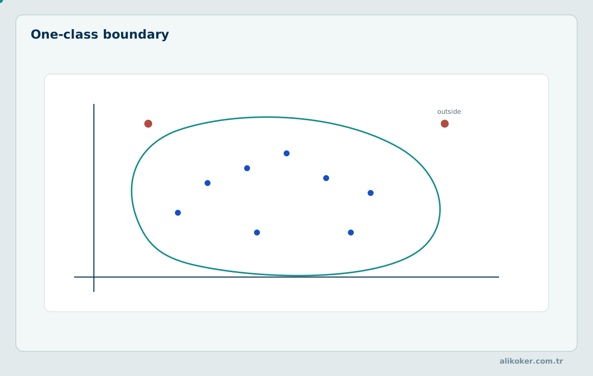
Deviation from a low-dimensional structure and departure from a learned support boundary are two powerful classical anomaly definitions. One relies on reconstruction residual, the other on support geometry.

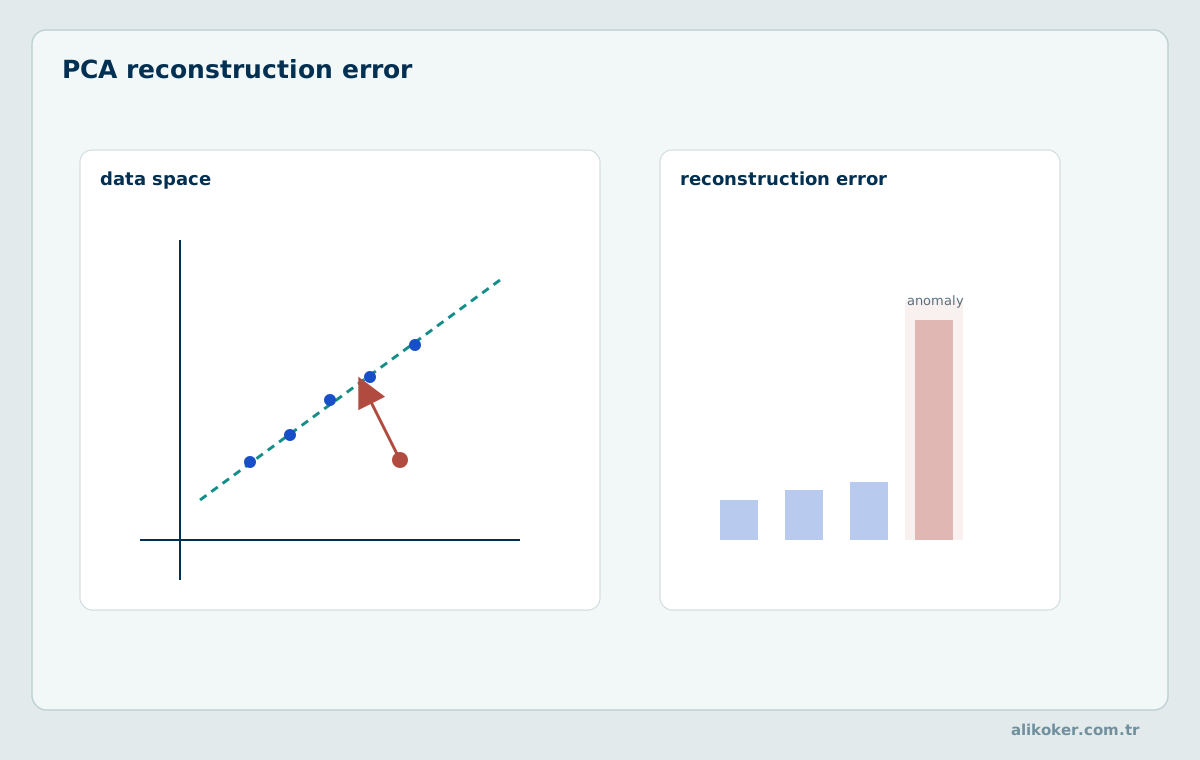
22.1. Unsupervised scoring

Unlabelled methods often score normality using density, distance, separability or clusters. Isolation Forest assigns higher anomaly scores to samples isolated by shorter random-tree paths. Local Outlier Factor compares local density with neighbours, which can help distinguish clusters of differing density.

22.2. One-class and probabilistic models

One-class SVM learns a boundary for the reference class but depends on kernel and hyperparameters. Gaussian mixture models approximate multimodal reference data, yet an incorrect number of components can cause normal operating modes to be flagged.

22.3. Clustering and high dimensionality

DBSCAN and HDBSCAN exploit density structure, but a noise-cluster label is not necessarily a system fault. In higher dimensions, distances may become less discriminative and irrelevant features can dominate scores. Scaling and feature selection must respect train–test separation.

22.4. Task-specific comparison

ML detectors require comparison under matched clean data, temporal splits, score thresholds and alert grouping. Success on one benchmark cannot establish general superiority. Interpretability matters when anomaly alerts must be audited.

22.5. Meaning of density- and isolation-based scores

Isolation Forest partitions observations randomly and tends to assign higher anomaly scores to points isolated by shorter paths. LOF compares local reachability density with neighbouring densities. One-Class SVM learns a boundary around a reference region. These scores have different numerical meanings and require calibration before sharing a decision threshold.

Feature scales matter especially for distance-based methods. Mixing millisecond latency with traffic volumes in bytes without suitable scaling can let one feature dominate. Scaling parameters must be fitted on the training period, not calculated from the evaluation data.

22.6. Threshold selection without labels

Without labelled faults, a threshold is often selected from a high quantile of scores on reference data. But contamination of that baseline incorporates true anomalies into the normal cutoff. Moreover, the 99th percentile roughly controls a 1% sample exceedance rate under the reference assumptions; temporal dependence means it does not guarantee a 1% independent event alert rate.

Thresholds must be evaluated with respect to distribution shift, unknown fault types and review capacity. Models should be compared on the same held-out events under the same alert-grouping policy, not solely through their own training scores.

Clustering, classification and representation learning build on Statistical Learning and Machine Learning: Classification, Regression, and Clustering.

Unit 23: Temporal Patterns and Subsequence Anomalies

23.1. Matrix profiles and discord subsequences

A matrix profile stores each fixed-length subsequence’s distance to its nearest nontrivial neighbour under the chosen normalisation. Large distances identify discord candidates. This detects unusual shapes even when individual samples lie within ordinary bounds.

23.2. Dynamic time warping

Dynamic time warping aligns patterns that evolve at different rates. Unconstrained warping may create physically implausible matches and increases computational cost. Distance and alignment constraints must be chosen together.

23.3. Forecast-residual detection

With x̂ₜ = f(xₜ₋₁,…,xₜ₋p), the residual eₜ = xₜ − x̂ₜ can be tested. Serially correlated residuals must not be treated as independent. Features computed using future observations produce unrealistically optimistic online detection performance.

23.4. Evaluating event onset

Detecting any point within an event is not equivalent to finding its onset promptly. Scoring an entire long event as correct after one positive sample can be misleading. Event-matching tolerance and missed-event costs should be fixed before evaluation.

23.5. Subsequence distance and window effects

A matrix profile stores each subsequence's nearest-neighbour distance among other subsequences. Large distances suggest unusual patterns. Window length m is critical: a short window can miss long patterns, while a long one can merge separate events. Constant subsequences require special handling during normalisation and distance calculation.

Z-normalisation compares shapes independently of amplitude, but may discard the very information that defines an amplitude surge. Raw-amplitude and normalised-shape distances can therefore be retained as separate scores.

23.6. Forecast residuals and seasonal anomalies

In a one-step forecast model, rₜ = yₜ − ŷₜ|ₜ₋₁ is the prediction residual. It should be judged relative to forecast uncertainty; error variance changes with forecast horizon. A model that has not learned a daily cycle can flag predictable daily peaks as anomalous. Conversely, a rapidly adapting online model may assign lower scores to a persisting true level shift.

Forecast-based evaluation must separate training and testing chronologically. Randomly shuffled time-series splits can leak information from the future into the reference model.

Unit 24: Deep Learning and Generative Models

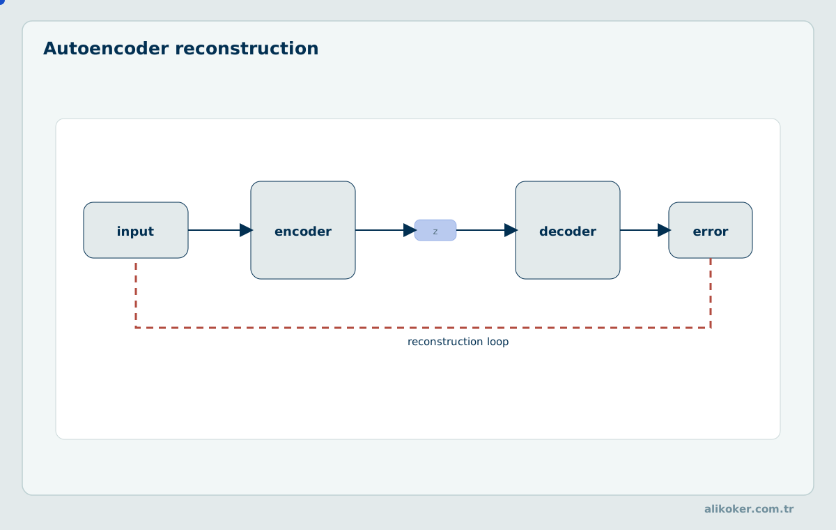
Models that compress and reconstruct normal patterns tend to produce larger residual errors on unusual samples.

24.1. Autoencoders

An autoencoder minimises a reconstruction loss L(x,x̂). If anomalies contaminate training data, it may learn to reconstruct them as normal. An over-capable network may accurately reconstruct many anomalous patterns, so score discrimination must be validated independently.

24.2. Recurrent and convolutional networks

LSTM/GRU architectures capture sequential dependencies, while temporal convolutions learn patterns within their receptive fields. Short windows may miss slow drift; long windows can increase latency and compute cost.

24.3. Attention and graph models

Transformer-based time-series models can capture long-range dependencies, with cost dependent on attention structure. Graph neural networks encode inter-component relations, but incorrect edges and temporal leakage can create spurious explanations.

24.4. Generative models and interpretability

VAE, GAN and diffusion approaches can model reference distributions or plausible reconstructions. Generated clean-looking data is not a recovered historical measurement. Variable contributions to alerts and reconstruction uncertainty should be reported.

24.5. Limits of reconstruction-error interpretation

An autoencoder maps input x through x̂ = D(E(x)) and scores a reconstruction loss L(x,x̂). A high error may indicate departure from training patterns, but a high-capacity model can also reconstruct anomalies well. A legitimate but underrepresented operating mode may generate high error. Near-identity mapping can make low reconstruction error uninformative about normality.

Using presumed-normal training data does not guarantee absence of faults. Feature units, channel weighting and temporal window length affect loss magnitude. Scores should be calibrated on validation data at an appropriate event level.

24.6. Temporal and graph models without causal overclaiming

Transformers and graph neural networks can learn long temporal dependencies and cross-channel relationships, but attention weights are not causal explanations. Two sensors may co-vary because of a separate physical fault; high learned association does not identify fault origin.

Low-latency online deployment needs a causal mask or equivalent past-only design. A bidirectional model trained using future context cannot simply replace an online detector without accounting for look-ahead latency. Large models should be benchmarked against statistical baselines using identical data and compute budgets.

Neural architectures and learning dynamics are treated more fully in Artificial Neural Networks and Learning Models.

Unit 25: Model Calibration, Drift and Reliability

25.1. Score calibration

An anomaly score of 0.95 does not necessarily mean a 95% probability of a true event. Probability interpretation requires calibration. For rare events, precision–recall curves and confirmed incidents per alert are informative.

25.2. Leakage and evaluation

Overlapping windows from the same device can leak near-identical patterns between training and test data. Splits must reflect event, device and time boundaries appropriate to deployment. Feature scaling is learned only from training data.

25.3. Distribution shift and retraining

Changes in normal behaviour can invalidate older thresholds and representations. Retraining should not be triggered solely by alert counts; data quality, labels and downstream performance need independent checks. Baseline poisoning by an adversary is a distinct risk.

25.4. Human review and auditability

In financial and forensic use, a model score alone cannot establish a verified finding. Decision records include input conditions, model version, explainable features and independent evidence. Abstention can be appropriate when uncertainty remains high.

25.5. Calibration, coverage and operating conditions

An anomaly score s(x) cannot be interpreted as P(event|x) without appropriate calibration. Where labelled validation data exist, probability calibration and reliability diagrams can be used, but rare-event calibration based on a handful of positives is highly uncertain. Sensitivity and specificity at a fixed threshold may not translate into the same operational performance when data collection or event prevalence changes.

Open-world systems encounter anomalies absent from training. An unknown regime should not be forced into a specific fault class with unjustified confidence. An uncertainty flag and review procedure are appropriate for novel events.

25.6. Selection bias in model retraining

In operational detection, only alerted records may receive detailed investigation. Labels from this subset do not represent non-alerted cases. 'Investigated and found benign' must not be treated as equivalent to 'never investigated' when defining negatives. Otherwise the model can enter a self-confirming feedback loop.

Sampling probabilities, label delays and verification sources should be retained for retraining. Analyst feedback must be tested on separate data before changing a production model, including checks for loss of recall on previously important event types.

Unit 26: Industrial Sensors and Mechatronic Systems

26.1. Sensor failure modes

Bias, slow drift, stuck-at output, saturation, intermittent disconnection and communication loss are distinct failure modes. A pointwise MAD test may miss a stuck sensor; derivatives, variance and independent reference channels provide complementary evidence.

26.2. Vibration and predictive maintenance

For rotating machinery, spectral peaks, sidebands and impulsive energy are examined together. Spectral kurtosis or envelope analysis can locate candidate fault bands. Load, speed and mounting conditions alter the baseline; increased vibration is not automatic proof of bearing failure.

26.3. Residual-based fault isolation

Multiple sensor channels can be checked against physical constraints. One deviating residual with otherwise consistent sensors may implicate a channel, while common-cause failures can affect all channels. Reliable isolation requires discriminative residual signatures.

26.4. Safe intervention

In safety-critical control, detection and shutdown decisions are separate policies. Measurement confidence, hazard severity, redundancy and safe-state design determine response. Analytical filtering must not conceal a physical hazard.

26.5. Sensor faults versus process faults

If one pressure sensor reads 2.5 bar while another in the same line reads 3.1 bar, there is an inconsistency, but neither reading is automatically correct. A third independent instrument, process model or calibration test is needed. Replacing a dissenting sensor by majority vote can fail under common-mode faults. Fault isolation depends on residual signatures and system observability.

Stuck-at, bias, drift, intermittency, saturation and gain faults produce different temporal patterns. Bias is an offset, drift grows slowly and stuck-at faults can create suspiciously low variance. Window length and statistic should reflect the physical fault mechanism.

26.6. Vibration spectra and condition-based maintenance

Bearing and gearbox faults often appear through frequency families, sidebands or envelope-spectrum changes rather than one large vibration sample. Harmonic frequencies move with rotational speed; order tracking can be more suitable than fixed-hertz thresholds. Load and mounting conditions also alter reference spectra.

A maintenance decision based on trends must consider fault criticality, inspection cost and the cost of unnecessary shutdown. A single elevated vibration sample does not identify fault location or establish remaining useful life.

Measurement uncertainty and calibration connect to Measurement Systems; physical sensor failure modes connect to Sensors and Sensing Systems.

Unit 27: Avionics, Navigation and Moving-Target Tracking

27.1. GNSS and inertial fusion

Inertial navigation supplies high-rate motion information while GNSS may provide an absolute reference. Outages, multipath and sensor biases challenge fusion. Measurement timestamps and covariance assumptions must be aligned in the estimator.

27.2. Innovation tests during manoeuvres

A real rapid manoeuvre can yield large NIS under a constant-velocity model. Automatically discarding the measurement may degrade tracking. Multiple-model filtering or bounded adaptation of process uncertainty may be appropriate with independent validation.

27.3. Redundancy and common-cause faults

Agreement between two sensors is not proof of truth when failures are dependent. Shared power, clock offsets or common interference can affect several channels. Fault-tree reasoning and probabilistic fusion assumptions must be aligned.

27.4. Safety and assurance boundaries

A statistical consistency test alone does not demonstrate airworthiness. Timing, behaviour under erroneous inputs, fault response and human interfaces require system-level verification against their own requirements.

27.5. Innovation and geometric consistency in navigation

GNSS/inertial integration may estimate position, velocity, attitude and sensor biases in one state vector. Innovation magnitude must be interpreted with satellite geometry, signal conditions and motion dynamics. During GNSS outages, inertial propagation continues but its uncertainty normally grows; a covariance remaining artificially fixed can signal a deficient uncertainty model.

Large innovations during a manoeuvre do not by themselves establish a satellite fault. GNSS quality indicators, dynamics limits, inertial sensors and competing hypotheses should inform measurement rejection. Filter comparisons require validated reference position and time alignment.

27.6. Limits of anomaly decisions in safety-critical systems

An anomaly score in flight control should not map directly to an actuator command. Detection, fault isolation, safety decision and control reconfiguration are separate auditable stages. False positives can disable a healthy control channel; false negatives can hide real faults. Fault tolerance and safe-state transitions cannot be specified by a statistical threshold alone.

In actual aircraft, certification, hardware failure coverage, timing bounds and development assurance govern deployment. Teaching examples illustrate methods and should not be presented as replacements for certified avionics logic.

Navigation integrity and flight-control constraints are discussed in Avionics Systems and Unmanned Aerial Vehicles.

Unit 28: Radar, Sonar and Target Detection

Adaptive thresholding accounts for local noise conditions rather than relying on one fixed threshold. CFAR is a standard illustration in radar detection.

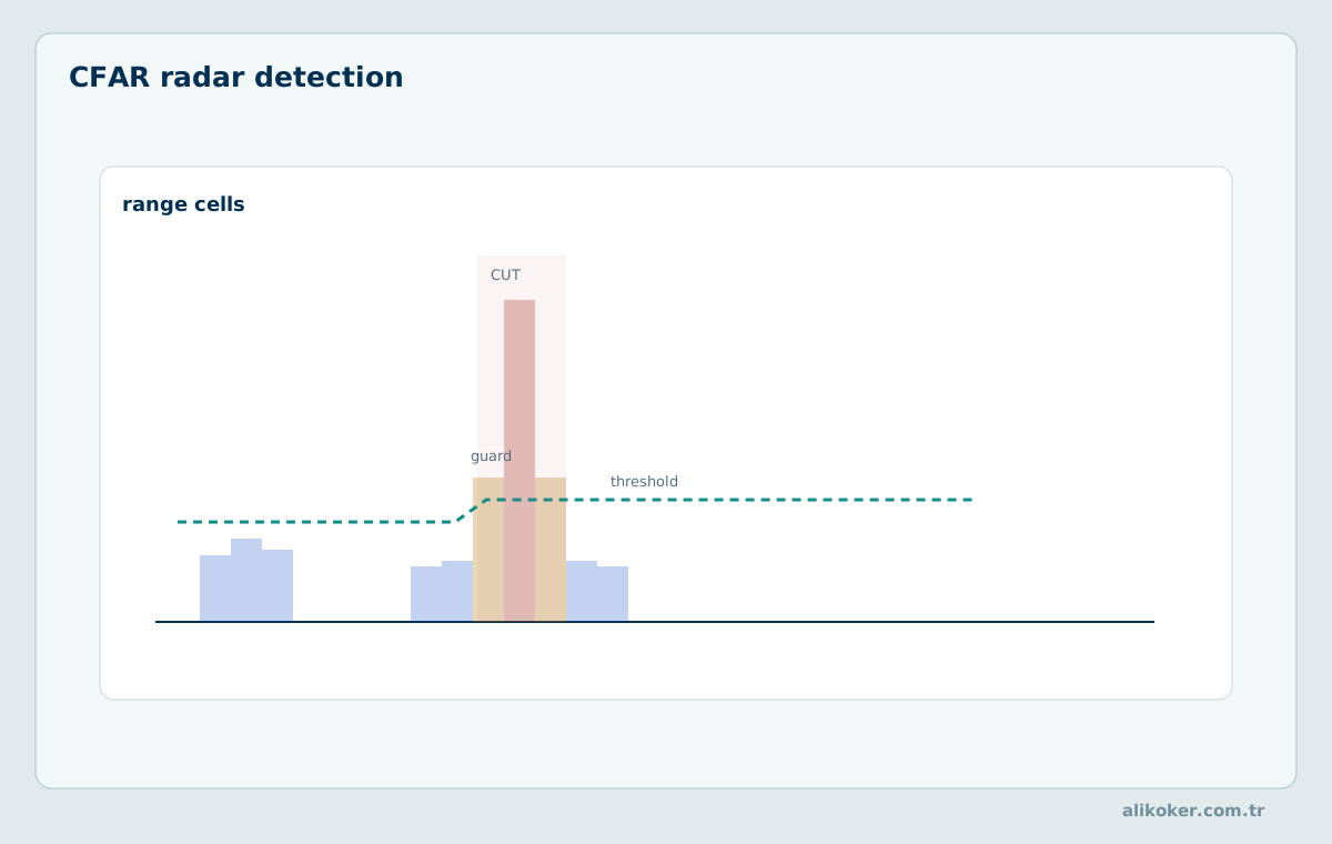
28.1. Signal and background models

Radar and sonar returns combine target echoes, environmental clutter, receiver noise and interference. A strong peak resembling a target is not necessarily a target. Receiver bandwidth, coherent integration and clutter statistics shape detection.

28.2. Matched filtering

For a known signal s(t) in the appropriate additive white Gaussian noise setting, a matched filter maximises output SNR under specified conditions. Template mismatch, Doppler shifts and coloured noise reduce performance. Its output still requires a detection threshold.

28.3. Constant false alarm rate

CFAR estimates local clutter from reference cells surrounding a cell under test. Cell-averaging CFAR works under reasonably homogeneous clutter, but multiple targets and clutter edges can corrupt its estimate. Guard and training cells must reflect range/Doppler resolution.

28.4. From detection to tracking

Detection generates candidates; tracking associates successive detections with physical objects. Incorrect association or missed observations can break track continuity even with sophisticated Kalman filters. State estimation and target identity are distinct problems.

28.5. Illustrative CFAR calculation

Suppose reference-cell powers are [2, 3, 2, 3, 2, 3, 2, 3], giving mean background power 2.5. Choosing an illustrative multiplier α = 4 yields threshold 10, and a cell under test with power 12 is flagged. A false-alarm probability cannot be inferred from α without specifying clutter statistics and the number of training cells.

28.6. Relationship between CFAR and local background

Cell-averaging CFAR estimates background power from training cells around the cell under test; guard cells limit target leakage into the estimate. With independent exponentially distributed power samples and N training cells, a threshold multiplier for the training-cell mean is α = N(P_FA^(−1/N)−1) under the corresponding assumptions. This expression is not universal: correlated clutter, nearby strong targets and background edges alter false-alarm behaviour.

Ordered-statistic CFAR may behave differently in multi-target or clutter-edge settings. The assumed noise distribution and resulting detection loss should be documented.

28.7. Matched filtering and sonar/radar event interpretation

For a known pulse shape s in white Gaussian noise, matched filtering correlates the observations with s to obtain the corresponding signal-to-noise-ratio gain. Doppler shift or time dilation can introduce mismatch. A high peak in a radar range–Doppler map is a target candidate, but may also arise from multipath, clutter or interference.

In sonar, environmental propagation, sound-speed profile and multipath affect timing and range estimates. A peak in one frame should not be treated as a confirmed target without track-level dynamic consistency.

Moving-target dynamics and flight applications connect to Avionics Systems and Unmanned Aerial Vehicles.

Unit 29: Seismic Events and Geophysical Signals

29.1. Components of a seismogram

A seismogram combines ambient noise, genuine wave arrivals, instrument response and anthropogenic vibrations. A rare earthquake onset is not noise to be removed simply because it is statistically unusual. Preprocessing can shift measured arrival times.

29.2. Short-term/long-term average ratio

STA/LTA compares energy in a short window with a longer baseline window. Window lengths depend on expected arrivals, sampling rate and ambient noise. Persistent vibrations or unrelated impulsive sources can trigger false detections.

29.3. Arrival picking and change detection

P- and S-wave onset estimates may use energy ratios, probabilistic change models or cross-station timing consistency. Event-detection confidence and arrival-time uncertainty should be reported separately.

29.4. Cross-station validation

An isolated spike at one station may be a local mechanical impact. Physically consistent travel-time delays across stations provide stronger evidence of a propagating event. Clock alignment and station geometry must be accounted for.

29.5. Short-to-long average ratio

If short-term mean energy is 12 and long-term mean energy is 3, STA/LTA = 4. An illustrative trigger threshold of 3 raises an event candidate. Nearby heavy vehicles, controlled blasts or interference may also produce the ratio. Earthquake interpretation uses arrivals and waveforms across other stations.

29.6. Physical interpretation of STA/LTA thresholds

Short-term and long-term averages in STA/LTA are often computed on absolute amplitude or squared signal energy. Their ratio R = STA/LTA flags a short-term energy rise above background. Event contamination of the LTA window can raise the baseline; an excessively short STA can trigger on random noise impulses. Different trigger-on and trigger-off thresholds can reduce repeated toggling.

Human activity or an instrument impact at one station can also cross the threshold. Earthquake interpretation requires waveform, arrival-time and multi-station travel-time consistency. Filtering can shift onset estimates, so its delay must be accounted for.

29.7. Distinguishing seismic waves from measurement artifacts

A seismic spike can arise from an earthquake, blast, vehicle, electrical interference or physical instrument contact. Travel-time-consistent arrivals across stations, coherence across components and local noise conditions help discriminate these causes. Automatic spike removal can irreversibly erase evidence of earthquake onset.

Arrival picking should distinguish the first detectable deviation from uncertainty in the physical phase onset. A noisy or faulty station can be downweighted in event location and magnitude estimation while its raw record remains preserved.

Unit 30: Anomalies in Audio, Speech and Power Systems

Short bursts, clicks and abnormal acoustic energy are often more legible on a spectrogram than on the raw waveform alone.

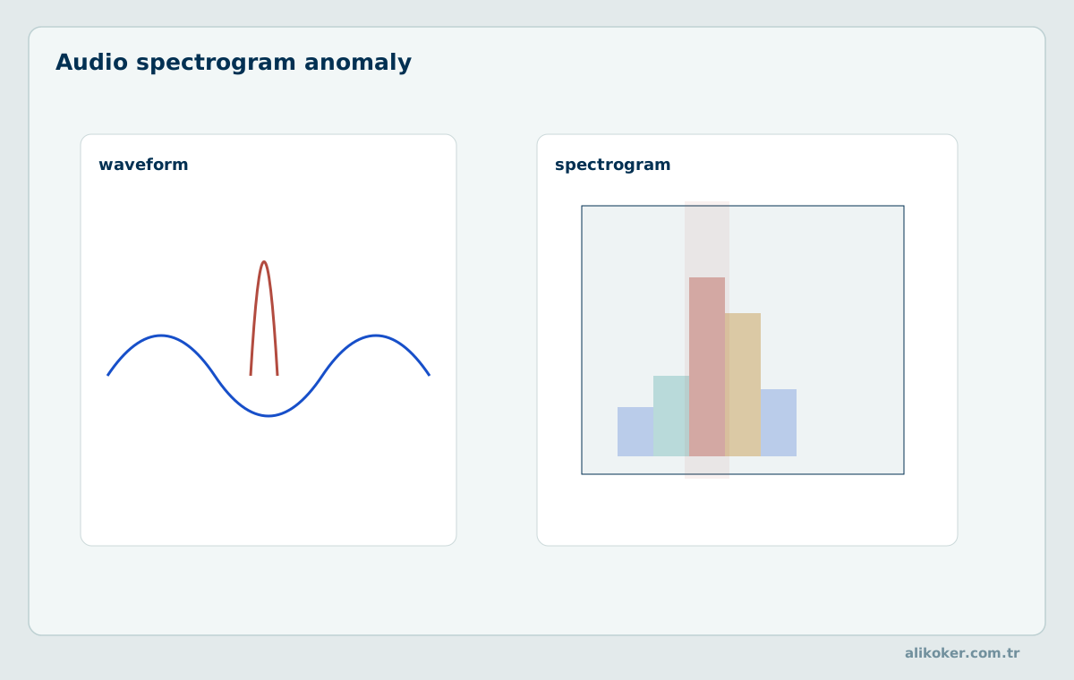
30.1. Acoustic events versus recording defects

Speech onset, an explosion or an instrument attack is a genuine acoustic event; a digital click, dropped packet or clipped waveform may be a recording defect. Spectral flux and short-time energy can rise in either case. Context and cross-channel consistency matter.

30.2. Harmonics and timbre

Upper harmonics contribute to timbre. Zero crossings, fundamental frequency, harmonicity and spectral envelope can be analysed jointly. Blind suppression of harmonics may damage intelligibility, sound quality or forensic features.

30.3. Power harmonics and transients

Nonlinear loads can inject harmonics relative to the 50/60 Hz fundamental. THD does not describe all power-quality events; dips, swells, flicker, impulses and interharmonics need separate treatment. The measurement window and point of common coupling must be specified.

30.4. Information preservation during correction

Improved audio or power-quality representations should not silently substitute for original observations. Frequency response, peak amplitudes, phase and timing shifts must be evaluated. Forensic audio requires explicit marking of derived versions.

30.5. Distinguishing acoustic harmonics from distortion

Higher harmonics of periodic audio can be intrinsic to the source. For fundamental frequency f₀, components at 2f₀, 3f₀, … contribute to timbre through their amplitudes and phases. Speech harmonics and vocal-tract formants are different concepts. A strong harmonic is not automatically distortion without context about source and recording chain.

Digital clipping can generate new spectral components as waveform peaks are truncated. Diagnosis can combine samples near the amplitude limit, waveform shape and spectral changes. Merely attenuating high-frequency energy does not recover the original recording.

30.6. Electrical transients versus steady harmonics

An inverter switching event can create a short voltage transient with broadband energy in an STFT window. A steady harmonic persists at integer multiples of the fundamental. Spectral leakage from a finite window can make a stable component appear as energy in adjacent frequencies.

Power-quality interpretation depends on RMS definitions, windows, harmonic grouping and measurement location. Acoustic and electrical harmonic analysis share Fourier mathematics, but their meaningful thresholds depend on different physical conditions.

Interpretation of acoustic impulses relates to Audio Processing and Forensic Audio Engineering; physical sources of electrical harmonics relate to Power Electronics.

Unit 31: Anomalies in Cybersecurity and Digital Forensics

Network behaviour is often judged against a baseline envelope. Volume bursts, direction changes and concentration together sharpen the event picture.

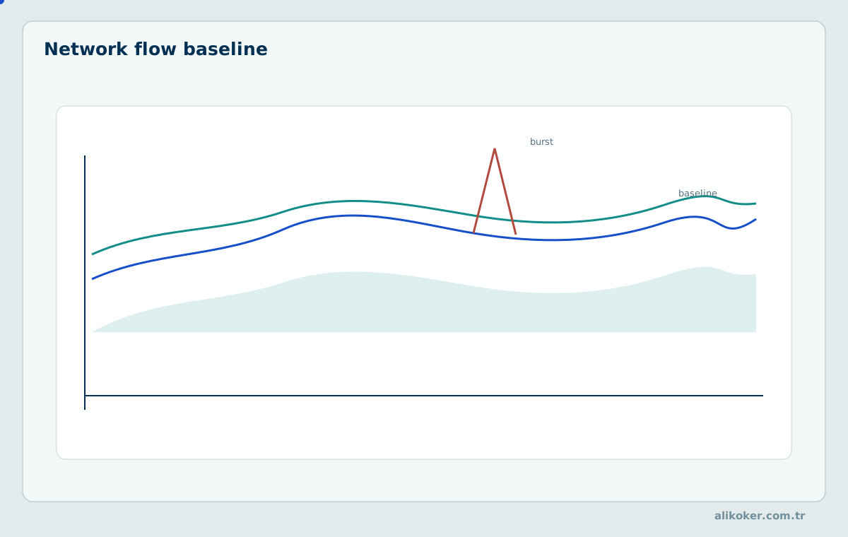
31.1. Network traffic and session behaviour

Packet rate, connection duration, destination diversity and privilege changes capture different abnormal behaviours. A surge may arise from maintenance, backup or attack. Permitted metadata and timing information can support statistical analysis even when payload content is encrypted.

31.2. Signatures, behaviour and event correlation

Signature detection recognises defined patterns, whereas behavioural detection flags departures from a baseline. Neither alone establishes intent or actor identity. Whether alerts belong to one incident must be checked using time, asset and action relationships.

31.3. Forensic integrity and timelines

Timeline reconstruction requires clock-offset and timestamp-resolution analysis. An unusual timestamp can result from corruption, clock changes, logging delays or a genuine event. Evidence provenance, raw records and computed anomaly scores remain distinct.

31.4. Operational cost of false alerts

Detecting rare attacks can overwhelm analysts with false positives. Alert grouping, prioritisation and human verification are part of the end-to-end detection system. Training only on previously investigated cases may create selection bias.

31.5. Baselines for network-flow anomalies

Packet counts, byte volumes, connection rate, destination diversity and session duration measure different aspects of network flows. Office start times, backups and software deployments can cause legitimate bursts. One pooled network baseline confounds these modes. Server role, protocol, hour and approved operational changes should condition the reference model.

A traffic surge may reflect DDoS, data transfer, misconfiguration or telemetry corruption. The anomaly score begins an investigation; attribution requires further network and host evidence. Automatic sanctions based on IP or user identifiers must account for false-positive impact.

31.6. Uncertainty in forensic event timelines

A mismatch between two logs can arise from clock skew, time zones, NTP adjustments, buffering or transport delay. An earlier timestamp in A than B does not necessarily establish physical event order. One unusual access or session pattern is not proof of abuse; integrity checks and alternative explanations are needed.

Forensic anomaly scores belong to an interpretation layer. Cryptographic integrity of raw records, chain of custody and derived event timelines are maintained separately. Normalisation should not silently overwrite original timestamps.

Network and security incidents connect to Cybersecurity Engineering, evidence integrity to Digital Forensics Engineering, and temporal interpretation of traffic records to HTS Analysis: Examining Traffic, Device, Time, Location, and Relationship Data from a Digital Forensics Perspective.

Unit 32: Anomalies in Economics, Finance and Business

32.1. Market movements versus bad data

Rapid price changes are neither automatically bad ticks nor proof of manipulation. Volume, bid–ask conditions, news and calendar context can help interpretation. Heavy tails and volatility clustering often invalidate simple Gaussian thresholds for financial returns.

32.2. Conditional variance and regimes

GARCH-type models represent conditional volatility changes. A fixed absolute-return threshold can over-alert during volatile regimes. Distribution, regime and forecast residuals should be considered together; no such model guarantees prediction of sudden market shocks.

32.3. Sales, inventory and supply chains

Demand spikes may reflect campaigns or seasonality. Sales anomalies require baselines conditioned on calendar, geography, stock availability and price changes. A drop in sales might be stockout rather than reduced demand; causal attribution requires additional data.

32.4. Business indicators

Operational indicators have different units and reporting frequencies. Combined risk scores require explicit scaling, dependence and missing-data rules. An anomaly threshold and management decision are separate stages with distinct cost and evidence requirements.

32.5. How context changes standardised deviations

Suppose Monday sales have mean 400 and standard deviation 40, while Saturday sales have mean 100 and standard deviation 20. An increase of 80 above each respective baseline gives z = 2 on Monday but z = 4 on Saturday. The same absolute departure has a different contextual rarity. Holidays and campaigns require further modelling.

32.6. Conditional volatility and price anomalies

Financial returns often exhibit time-varying variance. In GARCH(1,1), σₜ² = ω + αεₜ₋₁² + βσₜ₋₁² models conditional volatility. Under suitable positivity and stationarity conditions, past shocks affect expected future volatility. Thus the same absolute return may be exceptional in calm markets and ordinary during turbulence.

Residual distribution, parameter stability and sampling frequency must be assessed. An extreme return is not proof of a bad quote or unlawful trading. Exchange closures, dividends, splits and vendor revisions matter when constructing comparable price series.

32.7. Operational context in sales and inventory anomalies

Observed sales yₜ can depend on promotions, holidays, pricing and stock availability. During a demand surge, stockouts reduce recorded sales without implying reduced demand. Similarly, an inventory jump can follow returns, goods receipt or delayed bookkeeping. A detector should distinguish observed sales, latent demand and inventory movements.

A common demand shock across stores differs from a single-store deviation and requires a different operational response. Cross-sectional comparisons should condition on calendars and product-group relationships.

Turning business indicators into operational decisions connects to Decision Support Systems: Decision Analytics, Optimization, Uncertainty, and Decision Intelligence.

Unit 33: Financial Crime, Fraud and Corruption Indicators

Financial anomalies are not only about magnitude but also about structure. Unexpected centralization and unusual graph links are important red-flag patterns.

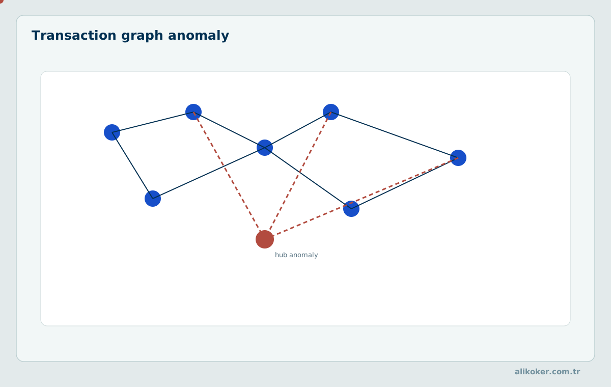
33.1. Suspicious transaction indicators

Transaction amount, frequency, counterparty network and apparent economic purpose may yield red flags. An unusual transaction is not necessarily illegal. AML review combines customer context, source of funds, relationships and applicable investigation procedures.

33.2. Public procurement and conflicts of interest

Repeated winners, low competition, split purchases or unusual party relations may warrant procurement review. Legitimate business explanations are also possible. Auditable risk indicators and independent verification must replace unsupported accusations.

33.3. Limits of Benford analysis

Benford’s law gives P(D=d) = log₁₀(1 + 1/d) for leading digits in suitable naturally scaled datasets. It does not automatically apply to narrow-range values, assigned identifiers or administratively bounded amounts. A mismatch is not evidence of fraud by itself.

33.4. Risk scoring and human investigation

With rare events, high sensitivity may still generate many false positives. Thresholds should account for investigation capacity and loss. Models trained only on previously investigated cases may inherit selection bias; review decisions and rationales should be recorded.

33.5. Leading-digit probability under Benford law

Under Benford’s law, P(D = 1) = log₁₀(2) ≈ 0.3010. This is a reference model for suitable naturally scaled datasets. It should not be applied uncritically to administratively bounded invoice amounts or assigned identifiers. A departure motivates review; it is not evidence of misconduct.

33.6. Conditions for proper use of Benford’s law

Benford’s law describes first significant-digit frequencies in suitable data-generating processes as P(D=d) = log₁₀(1+1/d), d = 1,…,9; for example P(D=1) ≈ 0.301. It does not apply to every numerical table. Narrow physical ranges, fixed-price schedules, assigned identifiers and bounded measurements may be unsuitable. Sample size and data acquisition mechanisms affect tests.

A departure from Benford frequencies is an audit indicator, not evidence of fraud. Data eligibility, test statistic and multiple-comparison controls must be documented. Many financial offences are better studied through relationships, timing and economic purpose than through digit frequencies.

33.7. Transaction networks and combining red flags

A graph with accounts, people and organisations as nodes and transfers or ownership as edges can reveal anomalies unrelated to individual amounts. Short cyclic flows, many-to-one transfers or unusual relationship clusters may merit review. Payroll, group-company transfers and legitimate payment networks can generate superficially similar structures; network context is essential.

FATF indicators can be more informative in combination, but one indicator does not establish an offence. Most labelled cases may have been selected for investigation, creating selection bias. Risk scores, review outcomes and legal findings must remain distinct.

Risk decision cost is addressed in Decision Support Systems: Decision Analytics, Optimization, Uncertainty, and Decision Intelligence, while the evidential limits of findings are addressed in Digital Forensics Engineering.

Unit 34: Software Architecture for Real-Time Detectors

In real-time detection, performance is not only accuracy; buffering, latency budgets and alarm timing are part of the design itself.

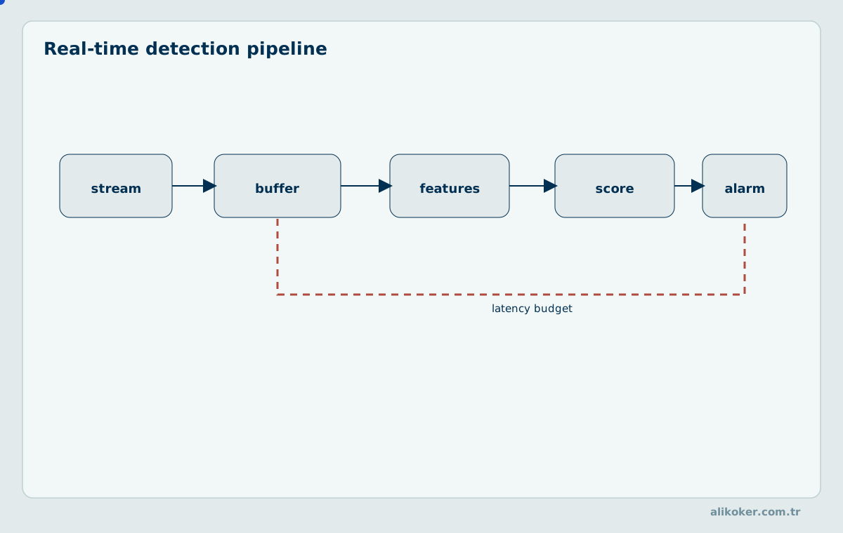
34.1. Causal fast path

Differences, thresholds, EMA and CUSUM can operate in O(1) time per sample with bounded state. Median/Hampel complexity depends on window data structures. Heavy models may run selectively after a lightweight screening stage, but end-to-end miss rates must be assessed.

34.2. Stream timing and latency

A centred odd-length W window requires about ⌊W/2⌋ future samples, giving lookahead delay ⌊W/2⌋Tₛ. Event-time versus arrival-time lag is separate. Queuing, filtering and inference times all contribute to end-to-end latency.

34.3. State isolation and concurrency

Each sensor or stream owns its history, state vector and alert state. Uncontrolled concurrent access can change results through races. Temporal order must be preserved within a stream, with explicit partitioning for parallelism across streams.

34.4. Fault tolerance and data integrity

Detector failure must not destroy original observations. Degradation policy should specify which expensive analyses may be skipped while basic integrity checks continue. Correction decisions, model versions and uncertainty must remain separable from the data.

34.5. Latency budget for a centred window

For a centred window of W = 21 samples at Tₛ = 5 ms, lookahead is ⌊21/2⌋×5 = 50 ms. Adding illustrative 20 ms queuing and 8 ms inference gives at least 78 ms. A system with a 60 ms deadline cannot use this configuration within its timing contract, regardless of detection accuracy.

34.6. Per-sample latency and memory budgets

A real-time detector can budget latency as L = L_ingest + L_window + L_compute + L_queue + L_decision. A centred 101-sample window at 1 kHz needs 50 ms of future data even with zero computation time. Causal EMA, difference and CUSUM updates can run at constant per-sample cost with bounded state.

Queue delay may remain low under average load but grow without bound during bursts. Throughput, p95/p99 latency, maximum queue depth, memory limit and drop/backpressure policy should be reported together. A strict deadline cannot be guaranteed by mean processing time.

34.7. State isolation and safe model versioning

State for each independent sensor or stream should retain its own last sample, filter covariance, control statistic and time reference. Concurrent out-of-order updates to one state object can invalidate the mathematics even when each operation is individually correct. Partition keys must identify the actual stream, and restart uncertainty and late-event handling must be defined.

Model and threshold changes must not obscure how past events were scored. Store model version, parameters and activation time; validate replacements through shadow evaluation or held-out data. A fail-safe design can preserve a lightweight detection path when a heavier ML component misses deadlines.

Queuing and latency budgets in high-throughput software systems relate to High-Performance Java Data Systems.

Unit 35: Experimental Design, Performance and Method Selection

35.1. Reproducible experimental data

Isolated spikes, persistent level shifts, gradual sensor drift, volatility clusters and genuine brief events require separate scenarios. Synthetic experiments should specify sampling, amplitude, duration, random seed and noise law. Real datasets need documented label provenance and unknown cases.

35.2. Pointwise and event-based metrics

Precision = TP/(TP+FP), recall = TP/(TP+FN). PR-AUC and false alerts per hour are informative for rare events. Scoring schemes that credit an entire long event after one correct point may mislead; onset delay and event matching must be defined in advance.

35.3. Measuring reconstruction quality

MAE and RMSE measure numerical estimation error; peak-amplitude error, timing shift and spectral distortion examine preservation of event information. A low RMSE after smoothing does not guarantee legitimate transients were retained.

35.4. Method selection criteria

Algorithm choice follows data distribution, temporal dependence, measurement model, operational loss, interpretability, compute budget and latency. No detector is universally best across domains. Comparative experiments must use matched splits, tuning budgets and resource limits.

35.5. Calculating classification metrics

With 45 true positives, 15 false positives and 5 false negatives, precision = 45/(45+15) = 0.75, recall = 45/(45+5) = 0.90 and F1 = 2×0.75×0.90/(0.75+0.90) ≈ 0.818. These metrics do not reveal detection delay, preservation of genuine peaks or alerts per hour; those outcomes need separate reporting.

35.6. Event-level evaluation and detection latency

Pointwise F1 can reward many correctly labelled samples in long events while hiding complete misses of short critical events. Event-level evaluation must specify matching between reference and predicted intervals beforehand. Onset tolerance, minimum overlap, duplicate-alert handling and event termination are part of the metric definition. Detection delay reported only for matched events must be accompanied by the fraction of missed events.

Methods should be compared on chronologically separated test data. False alerts per day cannot be inferred directly from a per-sample false-positive rate without accounting for dependence, event grouping and operating duration.

35.7. Correction quality and reproducible experiments

Given clean ground truth, MAE = (1/N)Σ|x̂ᵢ−xᵢ| and RMSE = √[(1/N)Σ(x̂ᵢ−xᵢ)²] quantify numerical reconstruction error. But the same method may halve a genuine transient peak. Peak timing, amplitude, spectral energy, event count and phase distortion also matter. Without clean reference data, true reconstruction error cannot be computed; only consistency or proxy measures can be reported.

Reproducible experiments record algorithm version, source split, anomaly injection procedure, random seed, thresholds, training budget and hardware. Results should be stratified by anomaly type and operating regime rather than claiming universal superiority from one average score.

Sampling and statistical inference connect to Probability and Statistics: Distributions, Sampling and Regression, and optimisation of review budgets to Operations Research.

References

• Charu C. Aggarwal. Outlier Analysis, 2nd ed.. Springer, 2017. https://doi.org/10.1007/978-3-319-47578-3

• Peter J. Huber; Elvezio M. Ronchetti. Robust Statistics, 2nd ed.. Wiley, 2009. https://doi.org/10.1002/9780470434697

• Michèle Basseville; Igor V. Nikiforov. Detection of Abrupt Changes: Theory and Application. Prentice Hall, 1993. https://web.mit.edu/fustflum/documents/papers/basseville.pdf

• Simo Särkkä; Lennart Svensson. Bayesian Filtering and Smoothing, 2nd ed.. Cambridge University Press, 2023. https://doi.org/10.1017/9781108917407

• Stéphane Mallat. A Wavelet Tour of Signal Processing: The Sparse Way, 3rd ed.. Academic Press, 2009. https://doi.org/10.1016/B978-0-12-374370-1.X0001-8

• Robert H. Shumway; David S. Stoffer. Time Series Analysis and Its Applications: With R Examples, 2nd ed.. Springer, 2006. https://doi.org/10.1007/0-387-36276-2

• Mark A. Richards. Fundamentals of Radar Signal Processing, 2nd ed.. McGraw-Hill, 2014. https://www.mheducation.com/

• Dhruba Kumar Bhattacharyya; Jugal Kumar Kalita. Network Anomaly Detection: A Machine Learning Perspective. CRC Press, 2014. https://www.routledge.com/Network-Anomaly-Detection-A-Machine-Learning-Perspective/Bhattacharyya-Kalita/p/book/9780429166877

• Suman Kalyan Adari; Sridhar Alla. Beginning Anomaly Detection Using Python-Based Deep Learning, 2nd ed.. Apress, 2024.

• Zahra Zohrevand; Uwe Glässer. Should I Raise The Red Flag? A Comprehensive Survey of Anomaly Scoring Methods toward Mitigating False Alarms. arXiv, 2019. https://arxiv.org/abs/1904.06646

• Miloš Resimić. Harnessing Artificial Intelligence (AI) for Anti-Corruption: Benefits and Challenges in Prevention, Detection and Investigation. U4 Anti-Corruption Resource Centre, 2025. https://www.u4.no/publications/harnessing-artificial-intelligence-ai-for-anti-corruption.pdf

• NIST/SEMATECH. e-Handbook of Statistical Methods: Generalized ESD Test for Outliers. NIST. https://itl.nist.gov/div898/handbook/eda/section3/eda35h3.htm

• IEEE Standards Association. IEEE Std 519-2022: Standard for Harmonic Control in Electric Power Systems. IEEE, 2022. https://standards.ieee.org/ieee/519/10677/

• Financial Action Task Force. The FATF Recommendations, revised June 2026. FATF, 2026. https://www.fatf-gafi.org/en/publications/Fatfrecommendations/Fatf-recommendations.html

• Varun Chandola; Arindam Banerjee; Vipin Kumar. Anomaly Detection: A Survey. ACM Computing Surveys, 2009. https://doi.org/10.1145/1541880.1541882

• Guansong Pang; Chunhua Shen; Longbing Cao; Anton van den Hengel. Deep Learning for Anomaly Detection: A Review. ACM Computing Surveys, 2021. https://doi.org/10.1145/3439950