Image Processing and Computer Vision Engineering

Digital image processing studies the transformation of radiation measurements into discrete images, their numerical processing, and the extraction of measurable properties. Computer vision seeks estimates of objects, motion, geometry, and scene state from those observations. Both disciplines require an explicit account of the assumptions under which inferred information remains valid. Sensor physics, digital signal processing, probabilistic estimation, optimization, and computer architecture therefore form a connected engineering foundation.

The measurement recorded by an imaging device must be distinguished from information inferred by an algorithm. Resampling a pixel, generating missing detail with a learned prior, and identifying a person are not equivalent operations: they respectively perform numerical transformation, estimation, and uncertain statistical decision-making.

Unit 1: Physical and Digital Foundations of Images

Digital imaging is grounded in optics, electromagnetism, geometry and sensor electronics. Light emitted or reflected by an object passes through the optical system, reaches the sensor, is converted into electrical quantities and is finally digitised into pixel values.

Digital Images, Pixels, and Resolution

A digital image consists of spatially sampled and quantized values. The smallest sample location is called a pixel. A pixel is not a physical point by itself; it is the result of the sensor element, optical spread, sampling geometry, and later numerical processing.

In a grayscale image, a pixel is commonly represented by one intensity value; in a color image it contains multiple channel values. With b bits per channel, up to 2^b numerical levels can be represented in principle. Greater bit depth reduces quantization step size at the cost of more data.

Spatial resolution is related to the horizontal and vertical number of samples, but more pixels do not automatically mean more real scene detail. Lens resolving power, focus, motion blur, sensor size, noise, and sampling conditions place an upper bound on the physical information captured.

This distinction matters in forensic imaging. Enlarging an image after acquisition does not create new sensor measurements; interpolation only calculates additional pixel values from existing samples.

Sampling and Quantization

Converting a continuous optical field into a digital image involves two distinct discretization steps. Spatial sampling determines where the scene is measured, while quantization maps each measured analog magnitude to a numerical level.

Insufficient spatial sampling can produce aliasing in fine patterns. Insufficient quantization can create banding and loss of subtle tonal detail. Optical low-pass behavior, sensor sampling geometry, and digital processing should therefore be considered as one acquisition chain.

“High resolution” is consequently not a single quality label that can substitute for pixel count, bit depth, and actual optical detail.

Light and colour

Visible light occupies a narrow region of the electromagnetic spectrum. A camera measurement depends on the source spectrum, surface reflectance, lens transmission and sensor sensitivity. RGB is common for acquisition and display, YCbCr separates luminance from chrominance, and Lab can be useful when perceptual distance matters.

The selected colour space affects thresholding, compression, colour constancy and similarity calculations rather than serving only as a display convention.

Optical system

Focal length, aperture, exposure time and sensor size jointly influence field of view, depth of field, motion blur and noise. Lens distortion changes measured image coordinates. Camera calibration estimates intrinsic parameters and geometric distortion so that image measurements can be related to physical geometry.

Human and machine vision

Human vision adapts to context and can infer structure from incomplete information. Cameras operate within limits imposed by dynamic range, exposure and spectral sensitivity. Infrared, thermal and high-speed sensors can nevertheless measure information outside normal human perception.

A pixel is therefore not the scene itself; it is the output of an optical, electronic and digital transformation chain. Understanding that chain is essential in metrology, computer vision and forensic image analysis.

From radiation to discrete measurement

An image is formed when radiation emitted or reflected by a scene passes through the optical system and reaches a photosensitive surface. The recorded value at a pixel depends not merely on the object's apparent colour but also on the illumination spectrum, surface reflectance, optical transmission, exposure time, and spectral sensitivity. A camera output is consequently not an invariant copy of the scene. In a simplified image-formation model, observed intensity is described by illumination and reflectance components; the distinction between shading and surface texture becomes difficult when these factors are entangled.

The ideal pinhole projection uses perspective division to map a three-dimensional point to the image plane. Real lenses introduce radial and tangential distortion, finite depth of field, defocus, and diffraction. Reducing exposure may limit motion blur while decreasing the number of captured photons and increasing relative noise. Increasing electronic gain does not create additional information about incident photons.

Sensor Calibration and Measurable Image Values

A pixel value is not a direct measurement of surface reflectance. Exposure, sensor gain, dark current, optical transmission, and illumination jointly determine the recorded signal. Under controlled exposure, a dark frame reveals electronic offset and hot pixels, while a uniformly illuminated flat field estimates sensitivity variation. A simplified correction is I_c = (I_raw − D) / max(F − D, ε), where D is the dark reference, F is the flat reference, and ε is a physically meaningful small denominator bound. This expression cannot be applied without qualification to gamma-encoded or otherwise nonlinear camera output.

A calibration pipeline establishes raw bit depth, black level, saturation limit, and colour transforms before acquiring references under comparable conditions. Defective pixels are detected, and correction quality is checked using measurements independent of the calibration inputs. Saturated regions do not contain recoverable intensity detail. For metrological and forensic use, the original image remains unchanged; linear measurement data and tone-mapped display output are stored separately.

Sampling, quantization, and resolution

The discrete image I[m,n] represents measurements at sampled spatial locations. Interpolation computes values between observations; it does not capture new scene information. If the spatial sampling frequency is insufficient for fine scene patterns, high-frequency components fold into lower frequencies, producing aliasing. Optical low-pass behaviour or explicit antialias filtering can suppress it, at the cost of limiting recoverable detail.

An ideal b-bit channel provides 2ᵇ numerical levels. For uniform linear quantization, the step is approximately Δ = (x_max − x_min)/(2ᵇ − 1). Treating quantization noise as white and independent requires assumptions about the signal or suitable dithering. Pixel count, bit depth, optical resolving power, and signal-to-noise ratio represent different performance dimensions and cannot be substituted for one another.

Sources of uncertainty

Dark current, read noise, photon statistics, defective pixels, saturation, and motion have distinct error mechanisms. Useful dynamic range depends on reliable measurement limits, not merely the numerical range of the file. When exposure, focus, colour encoding, and capture time differ, a difference image can reflect acquisition conditions rather than a physical change in the scene.

Unit 2: Image Representation, Colour, and Recording

Image recording converts sensor output into digital frames, reconstructs colour information, compresses the data and stores it as a file or stream. During transmission, the same data is additionally constrained by bandwidth, network delay and packet loss.

From sensor to frame

CMOS and CCD sensors convert photons into electrical charge. An analogue-to-digital converter turns that charge into numerical values. Colour filter arrays usually require demosaicing before full-colour pixels are available. Exposure, gain and white balance can alter pixel statistics before application-level processing begins.

Geometric and Radiometric Separation in Multisensor Records

Combining visible-light and thermal imagery requires three distinct operations: temporal alignment, geometric registration, and interpretation of measurement scales. Frame timestamps are first mapped to a common reference, lens distortion is corrected, and geometric correspondence is then estimated from calibration targets or shared structures. Equal pixel brightness is generally not a valid assumption across spectral bands; direct intensity minimization may fail. Edge or structural agreement and mutual-information criteria may be more suitable.

Resampling follows geometric warping. Nearest-neighbour interpolation preserves discrete label indices, whereas continuous intensities require an appropriate continuous interpolant. The effect of interpolation on the resolution of thermal measurements must be considered. Registration is not established solely by visually blending two frames: residual distances at held-out control points, depth-dependent disagreement, and capture-time offsets should be measured separately. A modest time offset for a moving target can resemble an error in the geometric model.

Codec and container

A codec defines how image or video samples are encoded and decoded. A media container organises one or more video, audio, subtitle and timing streams within a file or transport structure.

Lossless encoding preserves samples exactly but requires more storage. Lossy codecs reduce data volume by discarding selected information. Video codecs also exploit temporal redundancy across frames.

Live transmission

In live streaming, buffering and packetisation are as important as codec choice. Larger buffers can absorb network variation while increasing end-to-end latency. Long prediction structures improve compression efficiency but can slow recovery after packet loss.

A robust pipeline tracks resolution, frame rate, colour format, codec, timestamps and transformations together.

Colour spaces and numerical semantics

A single-channel image need not represent a calibrated physical luminance measurement. Colour samples depend on the chosen primaries, transfer function, and white point. Three-channel RGB values are not independent of the capture and display conditions. Representations separating luminance-like and chromatic components can improve compression or feature design, while perceptual spaces provide useful differences only within the validity of their colour-difference model.

Averaging values encoded by a nonlinear transfer function as though they were linear intensities produces incorrect physical blending. Linear-light processing requires conversion to a linear representation and re-encoding for output. Channel order, alpha interpretation, premultiplication, profile metadata, and full versus limited numerical range can introduce errors without causing a decoding failure.

Storage, compression, and timing

An image file contains encoded samples and interpretation metadata. Lossless compression seeks to preserve numerical samples, whereas lossy coding discards information through quantization or perceptual approximations. A video sequence adds frame timestamps, reordering, dropped samples, and possibly variable frame rate. Nominal frames per second does not establish the exact acquisition time of every frame.

Acquisition, colour conversion, resizing, compression, and transport should remain separately identifiable. Blocking artefacts, artificial edges, or colour displacement may originate from the encoding chain rather than the scene. Byte-level integrity and equivalence of decoded pixels are separate verification questions.

Unit 3: Spatial and Frequency-Domain Image Processing

Why DCT captures similarity

The success of DCT in similarity analysis does not come merely from moving the image into another coordinate system. It depends on which coefficients are selected and how they are quantized.

The library uses the upper-left 8 x 8 region of the 64 x 64 DCT matrix. This region carries:

• Mean image intensity
• Broad horizontal and vertical transitions
• Large object boundaries
• Overall light-dark distribution
• Coarse composition
• Low-frequency texture

Fine text, dense textures, compression noise, and single-pixel changes remain at higher frequencies. Excluding these coefficients from the digest makes the result more stable against small file-level changes.

Studies of similar DCT perceptual-hash approaches use standard-size reduction, selection of an 8 x 8 low-frequency coefficient region, and construction of a 64-bit value from these coefficients. Experimental work has shown that Hamming distance between perceptually similar images can be lower than between unrelated images.

The library does not store the absolute values of the 64 coefficients. It calculates their median and converts each coefficient into one bit according to whether it is greater than the median:

h_i = 1,  F_i > median(F)
      0,  F_i ≤ median(F)

The result is a 64-bit integer.

Using the median is important. The mean can be strongly influenced by outlying coefficients, particularly the DC component. The median represents the relative ordering of frequency coefficients. When overall gain changes, absolute coefficient values can change while their relative greater-than and less-than structure remains largely stable.

The perceptual digest therefore answers the following question:

"Do similar coefficients in the low-frequency structure of these two images remain on the same side of the median?"

This differs from pixel-by-pixel equality. Two coefficients can be numerically different and remain in the same class. A small change alters the bit only when it crosses the median threshold.

Two-dimensional convolution

For a linear, shift-invariant filter, Y[m,n] = Σᵢ Σⱼ h[i,j] · I[m−i,n−j]. Correlation differs by kernel reversal. Some implementations labelled convolution actually compute correlation; the distinction disappears for symmetric kernels. The sum of kernel coefficients determines the gain of constant regions. If h[i,j] = a[i] · b[j], a separable filter uses two one-dimensional passes, reducing arithmetic and often improving memory locality.

Zero padding, reflection, replication, and periodic continuation impose different assumptions at image boundaries. Sharpening may amplify both fine structure and noise, while smoothing attenuates spatial detail. Filter design must therefore account for the transfer response and error model rather than visual appearance alone.

Two-dimensional transforms

The discrete Fourier transform is F[u,v] = Σ(m=0…M−1) Σ(n=0…N−1) I[m,n] · exp[−j2π(um/M + vn/N)]. Its magnitude and phase convey different but coupled information; spatial placement and geometry depend strongly on phase relations. Multiplication in the frequency domain corresponds to convolution under appropriate boundary assumptions. Periodic extension can create edge artefacts, mitigated through padding or windowing.

The discrete cosine transform can concentrate the energy of spatially correlated natural images into a limited set of low-frequency coefficients. This property supports compression and approximate perceptual similarity, but a perceptual signature is not a cryptographic proof of file integrity. Hamming-distance candidate retrieval should be followed by stronger regional or geometric verification when the decision matters. Robustness to crop and rotation depends on the particular signature construction.

Complexity and precision

Direct k × k filtering of an M × N image requires approximately O(MNk²) operations. Separable filtering reduces the order to O(MNk); large convolution kernels can benefit from transform-based methods approaching O(MN log(MN)) under suitable conditions. Wall-clock time additionally depends on memory layout, vectorization, intermediate buffers, and data movement. Low-precision arithmetic requires analysis of overflow, rounding, and coefficient normalization.

Numerical Boundaries of Filtering

An identical convolution kernel produces different results under different image-extension rules. Zero padding can introduce artificial dark borders; reflection padding reduces abrupt transitions but does not create physical measurements outside the sensor field. Pixel type, saturation handling, and boundary assumptions must be specified for reproducible filtering. Computing directly in a narrow unsigned integer format may introduce overflow or rounding before the result is converted to the output type.

A separable k × k filter can use two one-dimensional passes of roughly 2k multiplications per pixel rather than k², provided that its kernel is separable. Transform-domain filtering can be advantageous for large kernels; transforms, temporary buffers, and padding often dominate for small frames. Measured end-to-end time and memory traffic, not arithmetic operation counts alone, determine a useful implementation.

Numerical example of transform-domain comparison

Consider a grayscale image rescaled to a common size and then represented using low-frequency cosine coefficients. The first coefficient of an orthonormal transform is closely associated with mean brightness; subsequent low-frequency coefficients describe coarse image structure. Comparing the first coefficient directly can increase sensitivity to global illumination changes. Thresholding selected coefficients around their median provides a compact binary signature. For two 64-bit signatures, d_H(a,b) = popcount(a ⊕ b), the number of set bits in their XOR result. Even a zero distance does not prove file integrity or object identity: distinct images can share a short signature.

A signature of b bits has only 2ᵇ possible outputs, far fewer than the number of possible images. Collisions are unavoidable. Fast candidate retrieval must therefore be followed by stronger verification when required. Decision thresholds should be calibrated on a representative validation distribution; cropping and projective transformations may require separate operating points.

Unit 4: Image Enhancement and Restoration

Image restoration estimates a cleaner image using information about the degradation process. Image enhancement, by contrast, usually aims to improve visibility or perceived quality.

Noise and blur

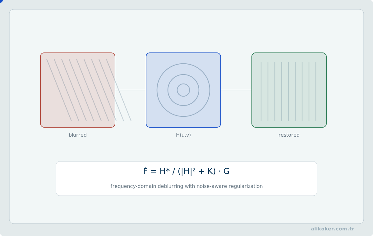
Gaussian, impulse and Poisson-like noise arise from different physical mechanisms. Median filtering works well for impulse noise, while other distributions call for different estimators.

Blur can result from defocus, camera motion or object motion. Wiener filtering and deconvolution methods estimate sharper content when the degradation function is sufficiently known. Blind deconvolution estimates both the image and the blur model.

Contrast and missing regions

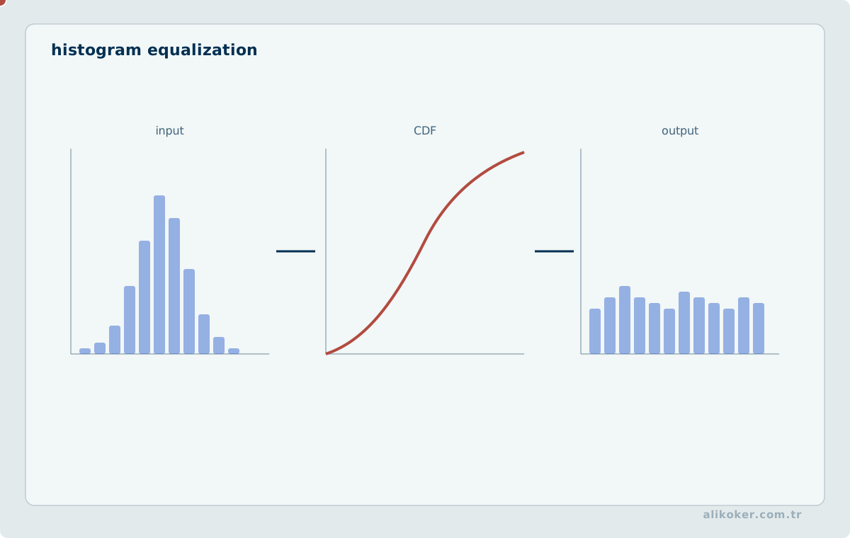
Histogram equalisation, gamma correction and local-contrast methods can expose low-contrast structure. Inpainting fills missing regions from surrounding structure or learned priors.

Details generated by a learned completion model are not direct measurements from the source image. Preserving the original recording separately from derived versions is therefore important in measurement and forensic workflows.

Super-resolution

Super-resolution estimates a higher-resolution representation from one or more lower-resolution observations. Pixel-oriented objectives usually produce conservative outputs, while perceptual or adversarial objectives may create sharper but more synthetic detail.

The value of restoration depends not only on appearance but also on whether measured information can be distinguished from estimated information.

Image Restoration as an Inverse Problem

An image affected by blur, noise, or missing samples can often be written as an inverse problem rather than as a sequence of arbitrary filters:

y = Hx + n,

where x is the unknown clean image, H the acquisition or degradation operator, n noise, and y the observation. The forward model explains how y would be produced from a known x; restoration attempts the reverse inference.

The inverse problem may be ill-conditioned. Small measurement errors can produce large solution changes, or several candidate images can explain the observation almost equally well. Data fit alone is therefore insufficient.

Regularization and Prior Information

Regularization balances agreement with the observation against assumptions about plausible image structure:

min_x  data_fit(Hx,y) + lambda * R(x).

R(x) may represent smoothness, sparse gradients, low rank, or a learned prior. If lambda is too large, real detail can be suppressed; if too small, noise and inverse-problem instability can dominate.

This provides a common view spanning classical Tikhonov/Wiener reasoning and modern learned or plug-and-play priors. Whatever the method, the assumption used to infer unmeasured detail should remain explicit.

Interpolation, Super-Resolution, and Real Detail

Interpolation estimates values between existing samples. Super-resolution aims to infer a higher-resolution representation from a lower-resolution observation and generally relies on stronger prior information.

Bicubic enlargement and learned super-resolution therefore make different claims. The first is a local resampling rule. The second can infer high-frequency structure learned from data. Such detail may look plausible without being identical to detail that was physically measured.

This distinction is especially important for forensic, scientific, or evidential imagery. Systems should separate measured pixel information from algorithmically inferred or generated detail and preserve the original data unchanged.

Observation and noise models

The model y = Hx + n distinguishes measured observations y, latent image x, degradation operator H, and uncertainty n. Photon noise may depend on the measured intensity, impulse noise produces sparse outliers, and speckle often has a multiplicative component. Applying the same mean filter to every noise type unnecessarily removes texture and edges.

Median filtering is robust against impulsive corruption, while edge-preserving nonlinear methods combine spatial proximity with intensity differences. Nonlocal estimators exploit recurring patterns. Comparisons of noise-reduction quality require consistent colour encoding, image scale, and compression conditions.

From a Noise Model to a Filtering Choice

Filtering begins by assessing the noise mechanism and spatial dependence. Rank filters can address impulsive corruption, locally linear estimators can suppress approximately additive stationary noise, and edge-preserving filters can weight both spatial and radiometric separation. Nonlocal estimators exploit the recurrence of similar patches but can erase fine structures when their similarity criterion is poorly calibrated. Multiplicative speckle noise should not be treated as independent additive noise without an appropriate transform or model.

A controlled experiment separates reference frames, corrupted frames, development data, and independent tests. Parameters are selected on development data; edge width, visibility of small targets, structural similarity, and processing time are then measured on held-out samples. A smoother output is not necessarily a better measurement when true edges have disappeared. For forensic examination, denoised frames are identified as derived images and never replace the original recording.

Inverse problems and regularization

A regularized inverse estimate may be written x̂ = argminₓ {||Hx − y||₂² + λR(x)}. The regularizer may favour smoothness, sparse gradients, or a learned image prior. An excessively large λ removes genuine detail; an excessively small value allows noise amplification. Naive spectral inversion becomes unstable near zeros of the blur transfer function. Regularized estimates reduce instability without recovering information that was never observed.

Multiframe super-resolution can exploit independent subpixel-shifted observations, unlike enlargement from one image. Single-image learned super-resolution uses a prior derived from training data and may invent plausible details. Scientific and forensic workflows must preserve the original record and keep measured, estimated, and generated details distinguishable.

Unit 5: Geometric Transforms and Image Registration

Projective camera model

For a homogeneous image coordinate p̃ = (u,v,1)ᵀ and world point X̃ = (X,Y,Z,1)ᵀ, the perspective mapping is s · p̃ = K[R | t] · X̃. Intrinsic parameters describe focal length and principal point; rotation and translation establish camera pose. Lens distortion requires separate calibration. Mapping world points into pixels is not identical to matching two uncalibrated images.

For a planar scene, or under particular pure camera rotations, p̃′ ∼ H · p̃ can relate two views. A single homography cannot generally align objects at different depths under camera translation because of parallax. An affine model excludes perspective deformation, but may have lower estimation variance when its assumptions are correct.

Robust estimation

Feature correspondence sets contain localization errors and false matches. Coordinate normalization improves the conditioning of linear estimation. Robust sample-consensus approaches fit candidate models to minimal subsets and evaluate geometric residuals across all correspondences. Pixel thresholds must be related to feature uncertainty and image scale. Repeating textures, moving objects, and degenerate geometry can still produce misleading agreement.

Multispectral registration may not satisfy brightness constancy: thermal and visible images represent different physical measurements. Mutual information, common edges, geometry, or cross-modal representations may offer more appropriate criteria. Independent control points and geometric residuals should be used to validate the resulting alignment.

An Operational Pipeline for Robust Registration

The geometric model must be selected before searching for a transformation. A planar scene or pure camera rotation may admit a homography, whereas parallax under camera translation generally prevents a single transform from describing the full image. After preparing comparable image representations, local features are extracted and paired using a distance appropriate to their descriptor type. Relative distance to the nearest competing candidate exposes ambiguities in repetitive textures; reverse-consistency checks reduce accidental matches.

A robust estimator draws minimal subsets to construct candidate transforms and evaluates reprojection residuals against thresholds informed by localization uncertainty. Degenerate samples, especially collinear or tightly clustered points, are rejected. The spatial distribution of inliers is more informative than inlier count alone. The accepted transform is re-estimated from consistent matches and tested on control points excluded from fitting. Direct photometric alignment may refine the result when texture and brightness consistency support it, but those assumptions cannot be transferred automatically to thermal-to-visible registration.

Identifiability of geometric estimates

A planar homography has eight independent degrees of freedom. Four suitably distributed point correspondences provide a minimal solution, but nearly collinear or spatially concentrated points can make the estimate ill-conditioned. Centering and scaling coordinates improves numerical stability in linear estimation. Conversely, low reprojection error does not prove that the observed scene is planar: few points, repetitive patterns, or systematically incorrect matches may also support an apparently consistent model.

For robust random sampling, let w be the independent inlier probability, s the minimal sample size, and p the desired probability of drawing at least one all-inlier set. The approximate number of trials is N = log(1−p) / log(1−wˢ). This relation assumes independent sampling and correct model structure. Correlated outliers or geometric degeneracy can degrade real performance.

Unit 6: Feature Extraction and Image Matching

Hamming distance and institutional scale

Similarity between two 64-bit digests can be measured with XOR and population count:

d_H(a,b)=popcount(a⊕ b)

The result ranges from 0 to 64. Zero indicates identical digests. As the value increases, differences in low-frequency structure increase.

This representation provides an important advantage for institutional systems. Each image is represented by only an eight-byte digest. Excluding database and index overhead, raw digests for one million images occupy approximately eight megabytes. Preliminary comparison of two images requires neither a high-dimensional feature vector nor image decoding.

This compact representation was important in the successful results I obtained in live use. Instead of reopening every image and comparing pixels or deep features across large datasets, DCT hashes could produce a fast candidate set.

The threshold is not universal, however. Acceptable Hamming distance must be determined for the data domain. Document images, face photographs, screenshots, and natural scenes do not have the same distance distribution. The correct threshold should be selected on a validation set containing positive and negative examples.

A linear scan costs O(M) for M records, but each comparison has extremely low fixed cost. At larger scale, the digest can be partitioned by selected bit regions, or multi-index search and approximate-neighborhood structures suitable for Hamming space can be used.

Image features transform raw pixels into representations that are easier to compare, index and classify. The objective is not only dimensionality reduction but preservation of task-relevant discriminative information.

Local and global descriptors

Global descriptors summarise the complete image through colour, texture or learned embeddings. Local descriptors represent neighbourhoods around selected keypoints. SIFT, SURF and ORB are classical examples of this approach.

Once an image is mapped to a feature vector, matching becomes a distance or similarity problem in representation space.

Similarity metrics

Euclidean distance, cosine similarity and Hamming distance suit different descriptor families. Binary descriptors naturally use Hamming distance, while normalised dense embeddings often use cosine similarity.

A matching pipeline may include preprocessing, keypoint selection, descriptor computation, candidate retrieval, geometric verification and thresholding. Methods such as RANSAC can reduce false candidates by enforcing geometric consistency.

Large collections

Linear scanning becomes expensive when millions of vectors are stored. Approximate-nearest-neighbour indices, quantisation and hierarchical search reduce query cost. Vector dimension also affects storage, cache behaviour and index size.

Feature extraction is therefore a representation problem designed jointly with the similarity metric and retrieval structure.

Repeatability versus discrimination

Feature detection identifies stable spatial structures; description converts their neighbourhoods into comparable representations. Corner scores often examine intensity variations in multiple directions. Scale-space analysis supports matching across apparent object sizes. Orientation normalization may improve rotational robustness, although additional invariance can reduce discriminative power.

For real-valued descriptors, a common comparison is d(a,b) = ||a − b||₂; binary descriptors admit Hamming distance. The nearest candidate alone is rarely sufficient evidence. Nearest-neighbour distance ratios, reciprocal matches, and geometric verification control false associations. Approximate nearest-neighbour methods trade search recall, memory footprint, and latency.

Candidate Search Followed by Geometric Verification

Descriptor representation dictates the distance function: bitwise mismatch counts for binary descriptors, and suitable vector norms or normalized inner products for continuous descriptors. A single similarity threshold does not transfer across representations; it must be calibrated against genuine and nonmatching pairs. Approximate-neighbour indexes can accelerate candidate search at scale but their recall, memory footprint, and build cost require measurement.

Retrieval scores alone do not demonstrate that two images depict the same structure. For selected candidate frames, local correspondences are tested under a consistent geometric transform. Evaluation separates image-level retrieval recall from the false acceptance rate of geometric verification. The dataset should include cropping, rotation, rescaling, compression, and low-contrast examples. Frames derived from the same source video must not leak across training and test partitions.

Perceptual signatures and retrieval

Global signatures provide inexpensive summaries; local descriptors are more effective when only parts of images overlap. Similar perceptual hashes do not establish byte equality. A two-stage system may generate candidates with a compact signature and verify them through regional correspondence or geometric consistency. This is often more economical than applying an expensive model to every stored image.

Validation should include repeated captures of the same object, visually similar distinct objects, and transformed or manipulated images. Tuning a decision threshold on the final evaluation set produces optimistic estimates. Candidate count, false positives, and workload-dependent response time must be measured at deployment scale.

Unit 7: Image Segmentation

Image segmentation assigns pixels or regions to meaningful classes. Unlike classification, the result preserves spatial location and can feed directly into measurement, inspection, medical imaging and scene-analysis pipelines.

Classical methods

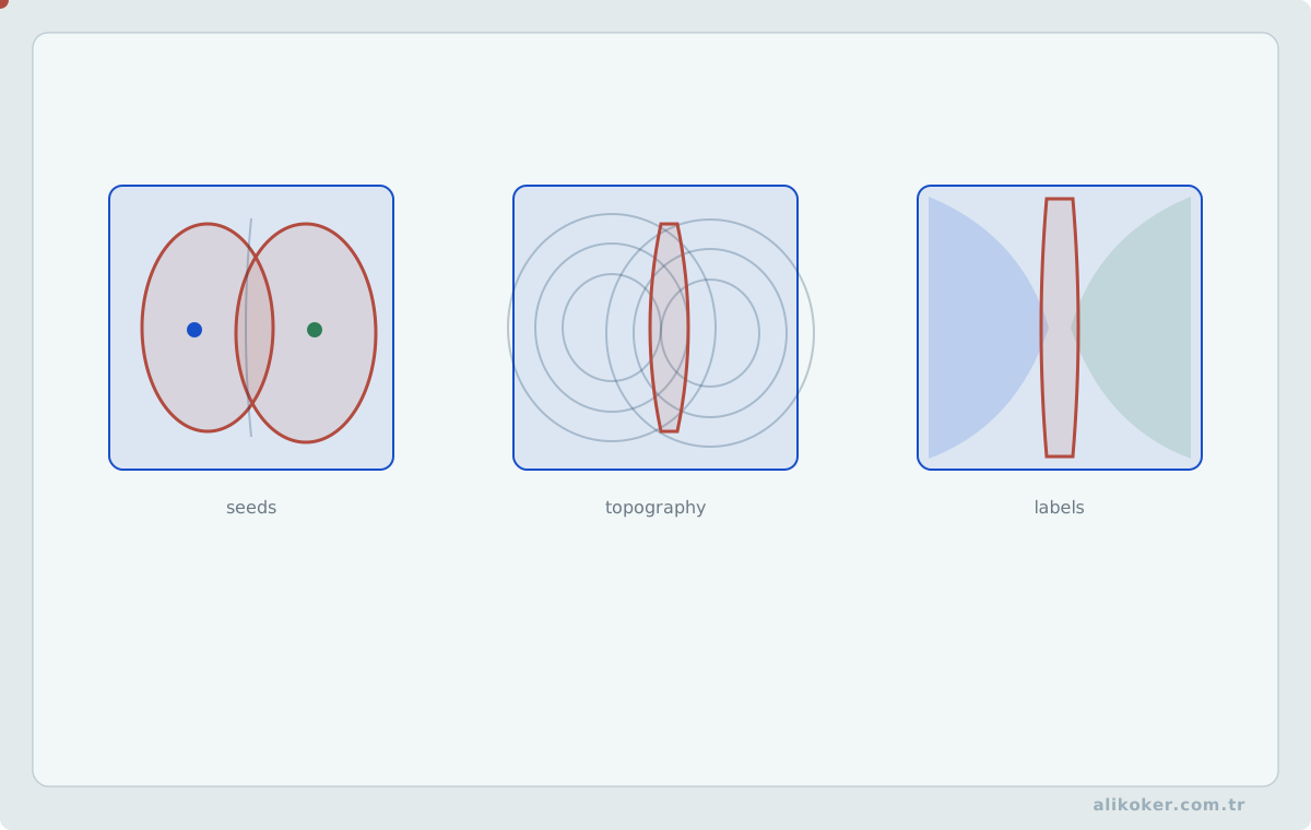
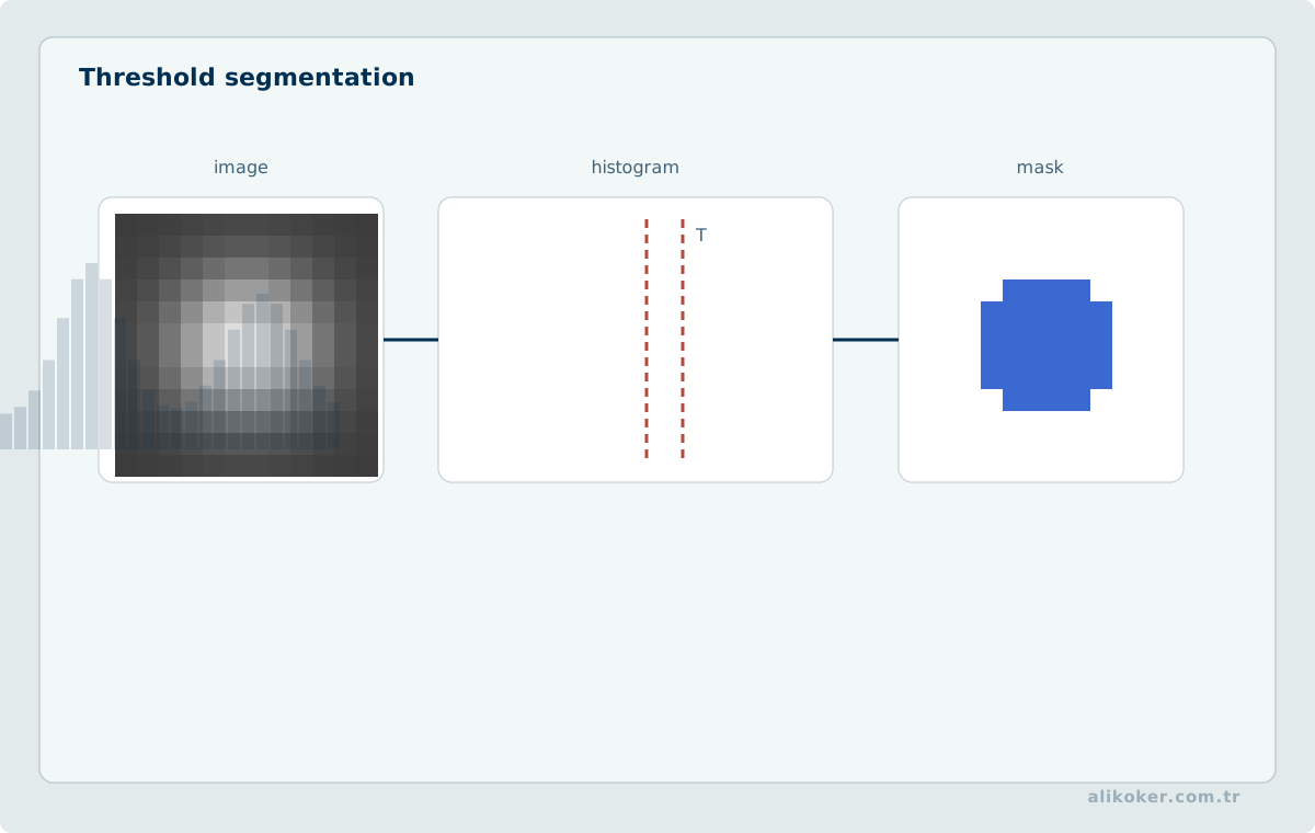
Thresholding separates regions according to intensity or another scalar feature. Global thresholds may work under stable illumination, while local thresholds are more robust under spatial variation. Otsu's method selects a threshold by maximising between-class variance.

Region growing, watershed and connected-component analysis provide more structural alternatives. Morphological opening, closing, erosion and dilation are commonly used to regularise masks.

Learned segmentation

Image segmentation is often implemented with encoder-decoder architectures such as U-Net. Semantic segmentation assigns class labels, instance segmentation separates individual objects, and panoptic segmentation combines both views.

Intersection over Union and Dice score are common overlap metrics. Pixel accuracy alone may be misleading when background pixels dominate.

Computation and annotation quality

High-resolution masks require substantial memory and computation. Tiled processing can preserve small structures but adds merge overhead. Inconsistent annotation boundaries also limit attainable model quality.

A segmentation mask is usually an intermediate representation consumed by tracking, OCR, measurement or another decision stage.

Segmentation levels

Segmentation assigns pixels to regions or object instances. Global thresholding is suitable when distributions are well separated; adaptive thresholding compensates for spatially varying illumination. Morphological opening and closing remove small structures or fill gaps, but the structuring-element scale may alter relevant measurements. Edge-based methods emphasize boundary consistency, while region-based methods favour internal similarity.

Semantic segmentation assigns a class per pixel; instance segmentation distinguishes different objects of the same class; panoptic segmentation combines class and instance information. In learned systems, annotation conventions, uncertain boundaries, and class imbalance directly influence observed performance. Missing a small critical object can be concealed by high global pixel accuracy.

Evaluation and geometric measurement

For binary regions A and B, IoU = |A ∩ B| / |A ∪ B| and Dice = 2|A ∩ B| / (|A| + |B|). Empty-mask conventions and multiple instances require explicit handling. Background-dominated pixel averages may hide errors; per-class and per-instance results are important. Boundary-distance metrics expose geometric inaccuracies that overlap scores may understate.

When segmentation drives physical measurement, pixel scale, perspective, calibration, and uncertainty must be propagated to the reported area or length. A visually smooth segmentation mask is not proof of dimensional accuracy.

Label Geometry and Boundary Errors in Segmentation

Pixel labels belong to the same coordinate system as the source image. Orientation correction, cropping, and scaling must be applied consistently to image and mask. Colour-coded class indices require an explicit mapping; linear interpolation of categorical masks creates invalid intermediate labels. Randomly dividing near-identical frames from a single recording across training and testing can substantially exaggerate reported performance.

High-resolution tiling must account for objects clipped at tile boundaries. Probability maps from overlapping tiles can be blended before applying a single final class decision. Region overlap and boundary displacement should be measured separately. A shift of only a few pixels has a greater proportional effect on narrow objects than on broad regions. Tests should cover lighting, compression, viewing angle, and scale, with object-level missed detections and false alarms alongside pixel-level scores.

Unit 8: Visual Pattern, Text, and Object Recognition

Visual pattern recognition converts recurring image structures into classes or symbols. Optical character recognition is a common example that combines image processing and language modelling within the same pipeline.

Visual representation

Classical systems normalise the image, extract edge, gradient or texture features, and classify them with methods such as k-NN or SVM. Convolutional networks can learn both representation and decision boundaries jointly.

OCR pipeline

Optical character recognition may include document orientation, text-region detection, line grouping, character or token recognition and language-aware decoding.

CTC, attention and Transformer architectures can map visual features to character or subword sequences. Perspective distortion, low resolution, complex backgrounds and unusual fonts directly affect performance.

Language information and traceability

Language models reduce ambiguity between visually similar characters. Keeping the raw OCR hypothesis separate from language-corrected output preserves the distinction between visual evidence and linguistic prior.

Character error rate and word error rate provide general measures. Critical fields such as dates, identifiers and names can be evaluated separately.

Object detection identifies both what objects are present and where they are located. Depending on the application, outputs may be bounding boxes, contours or masks.

Detector families

Two-stage detectors first generate candidate regions and then classify and refine them. One-stage detectors predict class and location in a single pass and are widely used in low-latency applications.

Small objects, dense scenes and high input resolution change the trade-off between computation and accuracy.

Overlap and post-processing

IoU measures overlap between predicted and reference boxes. When many candidates correspond to the same object, Non-Maximum Suppression removes duplicates according to confidence and overlap thresholds.

Boundary extraction can use gradient-based techniques such as Canny, active contours or instance-segmentation models.

Consistency Between Detection Data and Inference Coordinates

A detector operates on a transformed input frame. If its preprocessing resizes and pads the image, predicted bounding boxes must be mapped back through the inverse transform before they can be reported in original-frame coordinates. Otherwise a correct classification score may accompany an incorrect object location. Confidence thresholds, duplicate-box suppression, and minimum viable target size need calibration; a single operating threshold is rarely optimal for every class.

Annotation rules should define partially visible objects, heavy occlusion, boundary crossings, and uncertain classes before labels are collected. Hold-out evaluation must isolate recording sessions or acquisition conditions where possible, not merely different image filenames. Average precision integrates over score thresholds and cannot replace measured false alarms at the deployed operating point. Actual alert rate per camera, detection latency, and the effect of dropped frames should be evaluated separately.

Real-time performance

FPS alone does not describe end-to-end latency. Decode, resize, memory transfers, model execution, NMS and serialisation all contribute to total delay.

Throughput and single-frame latency should be measured separately, with target hardware and the surrounding data path treated as part of the detector system.

Classification and detection

Image classification estimates labels for a full frame; object detection also estimates locations and often multiple instances. One-stage and proposal-based detectors differ in candidate generation and computational cost. Bounding-box coordinates must be normalized consistently. Suppression of overlapping detections reduces duplicates, but can merge densely packed objects incorrectly.

Average precision depends on the intersection-over-union criterion, score ranking, and class population. Frames per second for model inference excludes capture, decoding, resizing, and postprocessing unless those stages are explicitly included. Whole-pipeline benchmarking prevents an overly optimistic real-time claim.

Optical character recognition

Text recognition involves detection, geometric correction, line representation, and sequence decoding. Perspective distortion, small glyphs, handwriting, compression, and low contrast change the error distribution. Language-based correction may substitute a plausible character for one that is not visually recoverable. Original image, raw recognition output, and corrected text must therefore be distinguishable.

Evaluation extends beyond aggregate classification accuracy to confusion patterns, missed instances, false detections, subgroup robustness, and probability calibration. Generalization to a new capture domain cannot be inferred from a single in-distribution test set.

Unit 9: Video, Motion, and Temporal Vision

Visual anomaly detection identifies observations that deviate meaningfully from a model of normal behaviour. Because future anomaly classes cannot always be enumerated in advance, the problem is often framed as one-class learning or modelling the normal distribution.

Modelling normality

Anomaly detection may use autoencoders, density estimators, one-class classifiers or distances in learned embedding spaces. A new observation receives a score based on reconstruction error, likelihood or representation-space distance.

The decision threshold depends on operational cost. The same numerical score can imply a different decision when false alarms and missed events carry different consequences.

Spatial and temporal context

A surface defect on a production line is mainly spatial. Behaviour in surveillance video may be anomalous only because of motion, timing or location. Optical flow, tracking and temporal encoders are useful in such settings.

False alarms and distribution change

Rare-event systems are sensitive to base rate: even a small false-positive rate may generate many alarms. Precision-recall behaviour and event-level costs are therefore useful evaluation measures.

Distribution shift occurs when normal deployment data moves away from the training distribution because of camera changes, lighting, seasons or operating regime. Anomaly scores are most useful when interpreted together with that context.

Lip reading, or visual speech recognition, infers speech content from temporal motion of the mouth and surrounding facial structures. It is primarily a temporal and multimodal signal-processing problem rather than a static image-classification task.

Visual speech signal

Lip, jaw and cheek motion correlates with speech production. Different phonemes may nevertheless produce similar mouth shapes, creating viseme-level ambiguity. Camera angle, frame rate, resolution, face coverings and illumination all affect the available information.

Visual speech recognition therefore depends on stable face and mouth-region tracking.

Temporal modelling

3D convolutions, recurrent networks, temporal convolutions and Transformers process motion across frame sequences. CTC or attention-based decoders can map visual features to character or token sequences.

Audio-visual fusion

Audio-visual speech recognition uses the visual channel as additional information when acoustic speech is degraded. Fusion may occur at feature, representation or decision level.

Accurate synchronisation is essential because camera and microphone clocks, buffering and transport delay can introduce temporal offsets between the two modalities.

Optical flow assumptions

Optical flow approximates the displacement of image brightness patterns between frames. Under local brightness constancy and small motion, Iₓu + Iᵧv + Iₜ = 0. This single equation cannot determine both velocity components without additional assumptions, such as local shared motion or spatial smoothness. Occlusion, illumination changes, large displacement, and newly revealed regions violate the simplified model.

Object motion and camera motion should be separated where possible. Residual flow after geometric stabilization can indicate independent motion, but parallax and registration errors also generate residuals. When timestamps are irregular, image displacement must be divided by actual elapsed time rather than a nominal fixed frame interval.

Multi-object tracking and visual speech

Tracking links detections across time. State estimation predicts object evolution; data association decides which observation belongs to which track. Temporary occlusion, reappearance, and identity switches are distinct failure modes. Position accuracy and identity continuity require different evaluation criteria.

Visual speech analysis extracts phonetic cues from lip motion, but distinct speech sounds can share similar visible articulations. Audio-visual fusion therefore depends on synchronization and modality reliability rather than assuming that visible mouth movements uniquely determine spoken words.

Prediction, Association, and Identity Continuity in Tracking

Multi-object tracking estimates state over time rather than classifying each frame independently. A state vector xₜ containing location and velocity can be predicted by xₜ|ₜ₋₁ = F xₜ₋₁, with uncertainty propagated through a covariance matrix. Simple centre distance ignores prediction uncertainty. A covariance-normalized innovation can reject detections incompatible with the predicted track. Eligible detections form an association-cost matrix from box overlap and appearance similarity; a global assignment step updates matched tracks and retains unmatched tracks for a bounded interval.

Discarding every low-confidence detection can fragment tracks under occlusion; a controlled secondary association pass can recover continuity. Such detections should not automatically initialize new identities, as this amplifies false tracks. Optical flow provides short-term motion evidence, although illumination changes and moving cameras violate a direct equivalence between flow and object motion. Trajectory analysis must normalize speed and direction for actual frame intervals. Pure coordinate-density clustering can mistake camera-dependent motion patterns for unusual behaviour. Identity switches, fragmentation, sustained tracking accuracy, and processing latency belong in the same evaluation.

Unit 10: Depth and Three-Dimensional Computer Vision

Depth estimation infers the distance of scene points from one or more visual observations. Stereo cameras, monocular models, structured light and time-of-flight sensors rely on different measurement principles.

Stereo geometry

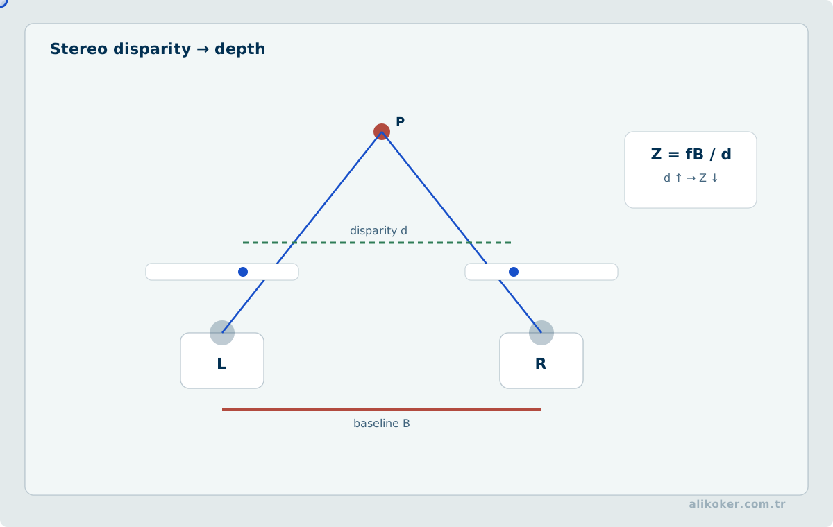
Stereo vision uses correspondences between two cameras observing the same scene from different viewpoints. In rectified images, the horizontal position difference of a scene point is called disparity.

Under a simplified pinhole model, depth is proportional to focal length and baseline and inversely proportional to disparity. Small disparity errors can therefore become large metric errors for distant objects.

Correspondence

Textureless surfaces, repetitive patterns, reflections and occlusions make correspondence difficult. Block matching, Semi-Global Matching and learned stereo networks provide different accuracy-computation trade-offs. Epipolar geometry constrains search to a line and reduces cost.

Monocular depth and sensor fusion

Monocular models infer depth from statistical cues such as perspective, object size, texture and occlusion. Absolute scale may require additional calibration or reference information.

LiDAR, radar and cameras can combine geometry with semantics when coordinate systems and timestamps are accurately aligned.

Epipolar geometry and triangulation

For two views, x̃′ᵀ F x̃ = 0 expresses the epipolar constraint. With known intrinsics, the essential matrix encodes relative rotation and translation direction, not absolute metric scale by itself. Three-dimensional points can be triangulated from viewing rays, although measurement noise prevents exact intersection. Small parallax and uncertain correspondence can sharply increase depth uncertainty.

For a rectified stereo pair, Z = fB/d, where focal length f is in pixels, baseline B is a physical distance, and disparity d is a pixel displacement. When disparity is small, one pixel of error may produce a large depth error. Monocular depth estimates use geometric or learned priors and may require additional calibration to establish absolute scale.

Error Propagation in Stereo Depth

A stereo reconstruction pipeline calibrates intrinsics and relative camera pose before rectification. After corresponding image points are constrained to common epipolar scanlines, matching costs are checked against texture ambiguity and occlusion. Left-to-right versus right-to-left disparity consistency can identify unreliable pixels. Only positive and sufficiently well-conditioned disparities provide meaningful metric depths.

For the simplified rectified stereo model Z = fB/d, depth error rises sharply as disparity decreases. First-order propagation yields |δZ| ≈ (fB/d²)|δd|. A one-pixel disparity error therefore produces a larger metric depth error for distant points than for nearby points. Depth maps should be accompanied by confidence or validity masks derived from matching consistency, occlusion evidence, and calibration uncertainty instead of treating every reconstructed value as equally reliable.

Multiview reconstruction

Joint optimization of camera parameters and scene points can minimize total reprojection error. Bundle adjustment depends on initialization, calibration, and the reliability of correspondences. Reconstructed points do not constitute a complete direct measurement of a scene: occluded regions, reflective surfaces, and low-texture areas retain ambiguity. Uncertainty should accompany geometric results where decisions depend on them.

Unit 11: Face Analysis and Biometric Vision

Face detection, person detection and face recognition are related but distinct tasks. Detection locates a face or person, while recognition evaluates identity similarity between an observed face and stored representations.

Detection and alignment

Haar cascades and HOG-based methods historically provided low-cost solutions. Modern learned detectors are more robust to changes in pose, scale and occlusion.

Facial landmarks can align the eyes, nose and mouth before recognition, reducing variation caused by crop position and head pose.

Embedding-based recognition

A recognition network maps the aligned face to an embedding. Samples of the same identity are encouraged to lie close together, while different identities are separated. Open-set systems must also support a no-match decision for people not enrolled in the database.

Face detection quality constrains every later stage. Poor cropping or alignment can shift the resulting embedding.

Biometric Decision Structure

Face recognition is one example of a biometric system. During enrollment, reference samples are converted into a template or feature representation; later samples are compared with that representation.

In verification, the question is whether a person is who they claim to be, typically producing a one-to-one comparison. In identification, the question is which enrolled identity best matches the sample, requiring a one-to-many search. As the candidate population grows, identification behaves differently in both computational cost and false-match risk.

A face image is first detected, assessed for quality, aligned, and converted into a feature vector. The resulting similarity score is not an identity by itself; a decision threshold must be selected according to the cost of false acceptance and false rejection in the application.

Because biometric traits cannot be replaced as easily as passwords, data protection creates an additional engineering obligation. Retention and access policies for raw images, templates, and comparison logs belong to the system design.

Evaluation

False-match and false-non-match rates should be interpreted together with the decision threshold. Camera type, pose, illumination, age and data distribution can affect these rates. Access control and data minimisation are also architectural requirements for identity-processing systems.

Detection, verification, and identification

Face detection finds candidate regions; alignment reduces pose variation using stable landmarks. Verification tests whether two recordings refer to the same identity, whereas identification searches a gallery or open-set population. These tasks require different operating characteristics. Closeness between embedding vectors is not a logical proof of identity.

False acceptance and false rejection depend on the threshold. Equal error rate marks one operating point and is not necessarily the appropriate threshold for a specific deployment. Open-set evaluation must measure rejection of unknown identities and erroneous assignment to registered identities. Time, pose, lighting, occlusion, and multiple samples per person should be reflected in dataset separation.

Robustness and forensic interpretation

Aggregate accuracy may conceal variation across acquisition conditions and populations. Presentation attacks and synthetic content introduce a threat distinct from ordinary matching errors. Thresholds require independent calibration; arbitrary similarity scores must not be presented as probabilities. For forensic comparison, sample quality, a relevant reference population, and competing explanations constrain the strength of any identity statement.

Operating Points in Biometric Evaluation

Face detection, geometric alignment, representation extraction, and score thresholding create distinct error sources. Limited resolution, pose variation, occlusion, and compression alter the representation. A low score does not necessarily demonstrate different identities, and a high score is not definitive proof of identity. Similarity scores cannot be interpreted as calibrated probabilities without a specified population and acquisition process.

Genuine and impostor score distributions should be measured on data whose identities are isolated from training. The true-match rate at an explicitly bounded false-match rate defines an operational point. As the gallery grows, even a modest probability of false acceptance in one comparison can produce a material probability of at least one spurious candidate. Error disparities across acquisition conditions and population subgroups require separate evaluation. Synthetic imagery and edited faces demand provenance checks independent of the matching score.

Unit 12: Image Generation, Reconstruction, and Manipulation

Image generation covers a broad family of methods ranging from geometric resampling to learned generative models. Their common property is that the output is derived from existing data or a learned distribution rather than directly measured by a sensor.

Resampling

Nearest-neighbour, bilinear and bicubic interpolation compute samples on a new grid. Scaling, rotation and geometric correction transform existing information but do not automatically recover physical detail that was never captured.

Generative models

Autoencoders map inputs to compact latent representations. Variational autoencoders introduce probabilistic structure into that space. A generative adversarial network trains a generator and discriminator with opposing objectives.

Diffusion models learn to reverse a gradual noising process and can produce highly realistic samples. Realism does not imply that the generated content was present in an original scene.

Synthetic data and identity transfer

Synthetic data can expand rare classes and reduce the cost of physical data collection. Synthetic artefacts may nevertheless become shortcuts learned by downstream models.

Face replacement, identity transfer and reenactment require explicit provenance management. Visual realism, geometric consistency and content provenance are different properties.

Evaluation should therefore include provenance, labelling, model version and the points at which synthetic and measured data interact, in addition to visual quality.

Quality and limits in geometric resampling

Nearest-neighbor, bilinear, and bicubic methods are not merely different "quality settings" for resizing or geometric transformation; they encode different local reconstruction assumptions. Without anti-alias filtering before reduction, high-frequency content can fold into false lower frequencies. Enlargement, meanwhile, cannot measure physical detail that was absent from the source samples.

Inverse mapping makes it natural to map every destination pixel back to a source coordinate and reduces holes. Repeated resampling, however, can accumulate blur or ringing. When possible, several geometric transforms should be composed and the original source sampled once.

Quality in reconstruction and generation pipelines is not captured by pixel similarity alone. Geometric fidelity, aliasing, edge structure, color consistency, and task-specific perceptual measures may all matter.

The boundary between reconstruction and generation

Reconstruction attempts to infer a missing or degraded quantity from observed data and an explicit or implicit acquisition model. Generation can create content that is not uniquely determined by the observation.

The same model family can be used for both tasks; the distinction lies in the epistemic claim, not the model name. A diffusion model can perform super-resolution or free-form generation. In the first case the output is conditioned on an observation, yet some high-frequency detail may still originate from the model prior.

A trustworthy computing pipeline should therefore make traceable which information was measured, which was deterministically transformed, and which was estimated or generated by a model.

Interpolation and generative inference

Nearest-neighbour, bilinear, and cubic interpolation calculate new sample positions from observed values. Learned single-image super-resolution estimates missing frequencies using a prior drawn from training data. Generative approaches can construct scene-consistent details that were never present in the recorded scene. Visual sharpness is therefore not equivalent to evidential accuracy.

Pixelwise reconstruction losses and perceptual objectives measure different kinds of similarity. A low pixel error may look blurred, while a perceptually convincing image may contain structures unsupported by observations. The choice of objective must follow the reliability requirements of the application.

Traces of modification

Cropping, rescaling, compositing, localized editing, and recompression affect different statistical traces. A boundary mismatch or compression inconsistency is an indicator to examine, not conclusive proof of manipulation. Legitimate processing and platform conversions can produce similar patterns. Detection performance must be characterized by edit type and by both false-positive and false-negative error rates.

Unit 13: Forensic Image Examination

Provenance and integrity

The original file is preserved while acquisition, copying, transformations, access, and analytical actions are documented. A cryptographic digest can verify byte integrity but does not establish whether the scene depicted actually occurred. Metadata can support an analysis but may be editable, absent, or incorrect. Sensor traces, lens characteristics, and coding patterns are probabilistic source evidence that require a representative reference set and consideration of alternative explanations.

Validation and reporting

Forensic enhancement should be distinguished from presentation-oriented editing. Contrast adjustment or restoration may help inspection, but newly visible edges need not correspond to physically recorded boundaries. A reproducible report describes source files, transformations, parameters, validation samples, limitations, and observations. Inferred or generated details are not new measurements.

When hypotheses are compared, the test population and error characteristics must correspond to the relevant conditions. Uncalibrated similarity scores cannot support categorical conclusions. Independent methods may strengthen a finding, but their shared failure mechanisms must also be considered.

Comparing sensor and compression traces

Fixed-pattern noise and pixel-response nonuniformity may provide weak clues about acquisition hardware, but separating these traces from scene content is difficult. Sensor-fingerprint methods require representative reference captures to estimate shared components; identifying a source from one image carries different statistical limitations. Smooth scenes, low exposure, heavy compression, and extensive postprocessing can obscure sensor traces. Demosaicing artefacts and colour-filter-array patterns also depend on the acquisition pipeline.

Repeated lossy compression can produce periodic structure in transformed-coefficient histograms; absence of that pattern does not establish absence of editing. Likewise, different compression characteristics across a frame cannot, by themselves, establish intent. Interpretation requires suitable controls from comparable devices and known encoding settings. Observations, plausible alternative processes, and the validated domain of the inference must remain distinct.

Comparable Experiments in Image Forensics

A questioned recording is first preserved at the byte level, with format inspection, metadata extraction, and an immutable original. Competing explanations are then examined separately: block boundaries and compression traces can suggest transcoding; local differences in sensor noise may reflect different acquisition or processing; regular interpolation patterns may indicate geometric resampling. None proves deliberate manipulation on its own. Legitimate enhancement, exposure correction, and transmission can produce overlapping traces.

Reference experiments should use known originals and controlled modifications from comparable capture pipelines whenever possible. Samples used for score selection must be kept separate from those used for final assessment. The report distinguishes measured observations, processing parameters, alternative causes, and limitations of inference. A numerical threshold calibrated under a different camera or compression distribution cannot be transferred without new validation.

Unit 14: Real-Time Vision and Production Engineering

End-to-end timing

Vision-system latency comprises acquisition, decoding, transformation, inference or filtering, postprocessing, and communication. Low model execution time does not ensure low end-to-end latency when frames queue or traverse networks. If arrival demand persistently exceeds service capacity, backlog accumulates. Real-time operation need not process every frame; frame-dropping policy, freshness, and timestamp fidelity should be explicitly specified.

Memory, concurrency, and validation

Image stride, alignment, channel depth, and layout affect filter performance. For low-arithmetic-intensity stages, memory bandwidth or data copies can dominate computation. Parallel implementations need defined buffer ownership to avoid races; accelerator transfer overhead may outweigh the benefits for small batches. Quantization and pruning change quality unevenly across data distributions, requiring measured accuracy-latency curves.

System validation should include high-resolution frames, variable frame rates, malformed media, concurrent streams, long-running operation, and backpressure. Tail latency and queue occupancy complement mean processing time. Input versions, processing order, software versions, and execution environments support reproducible benchmarking.

Time and Buffer Ownership in Frame Pipelines

Equal average arrival and service rates do not prevent burst-induced queues. Capture, decoding, geometric preprocessing, inference, and postprocessing each contribute service time and buffering. Queue bounds and memory ownership must be explicit. Double buffering can reduce copies, but a producer must not overwrite a buffer still being read. With asynchronous accelerator transfers, reusing storage before the completion signal risks silent corruption.

For live tracking, an unbounded queue of stale frames is usually less useful than a declared maximum acceptable result age. Dropping outdated frames must be reflected in the time step of the tracking model; assuming uniform frame intervals under irregular delivery biases motion estimates. Evaluation should report warmed-up end-to-end p50/p95/p99 latency, frame age, drop rate, peak memory, and task accuracy together. An optimization is valuable only if it improves the freshness and reliability of the output, not merely model throughput.

References

• Digital Image Processing. Fourth Edition. 2018.
• Computer Vision: Algorithms and Applications. Academic draft dated 2010; foundational theoretical sections.
• Multiple View Geometry in Computer Vision. Second Edition. 2004.
• Understanding Deep Learning. 2023.