Image and Audio Processing

An engineering view of digital image and audio processing, from sensing and sampling to feature extraction, learned models and real-time constraints.

Image and audio processing deal with transforming physical signals into digital representations and extracting useful information from them. Cameras produce spatial samples, while microphones produce time-dependent samples. Their data structures differ, yet both domains share core ideas such as sampling, quantisation, noise, filtering, spectral analysis and feature extraction.

Digital signal chain

A processing pipeline may include sensing, analogue front-end circuitry, digitisation, preprocessing, representation, modelling and decision stages. Input quality constrains every stage that follows, so model accuracy alone does not describe system quality.

The sampling theorem defines the limits under which continuous signals can be represented by discrete samples. The Fourier transform provides a frequency-domain view of the signal. Edges and texture in images, and formants or spectral energy patterns in audio, can become easier to analyse through these representations.

Classical and learned methods

Classical techniques rely on explicit operations such as filtering, thresholding, morphology, correlation and geometric transforms. Learned systems derive representations and decision boundaries from data. Practical systems often combine both. An image model may depend on resize and normalisation stages, while a speech model may receive VAD-filtered log-Mel features.

System metrics

Accuracy should be considered together with latency, throughput, memory use, model size, energy consumption and data movement. Offline forensic analysis and interactive real-time processing have different performance envelopes.

Multimodal learning combines image, audio and text through shared or related representations. It becomes valuable when one sensor or modality contains incomplete evidence.

Image and audio processing are therefore end-to-end information-processing problems extending from physical acquisition to the final decision.

Topic Map

I keep the image-and-audio material as a connected set of notes rather than one oversized article. Optics and acquisition, feature extraction, restoration, segmentation, recognition and forensic use each have their own page; the map below shows how those narrower notes fit together.

Image

Audio

Cross-domain applications

Academic origin

One academic foundation of this topic cluster is the chapter Image and Audio Processing, written with Nursel Yalçın and published in the 2022 book Artificial Intelligence - From Theory to Practice. The web entries are not copies of the chapter; they separate the subjects into reference pages and extend them with current technical links and applied engineering context.

Resampling, Geometric Transforms, and Interpolation

During image enlargement, reduction, rotation, perspective correction, or geometric registration, a destination pixel usually maps to a noninteger source coordinate. A geometric transform therefore contains two distinct problems: find where to sample and estimate the sample value at that location.

Forward mapping sends source pixels toward the destination and can leave holes or map several sources onto one output. Raster pipelines therefore often use inverse mapping: each destination pixel is mapped back to a source coordinate and sampled there.

Common choices include:

nearest-neighbor: minimal cost and useful for categorical labels because it invents no intermediate labels, but it can look blocky;
bilinear: combines four neighbors with separable linear weights, giving smoother but sometimes softer output;
bicubic: uses a wider neighborhood for smoother variation, at greater cost and with possible overshoot or ringing.

Interpolation during enlargement does not create genuine new detail; it applies a reconstruction assumption between existing samples. Reduction has an additional requirement: high spatial frequencies that cannot be represented at the new sampling density should be suppressed before decimation or aliasing may occur.

Zoom quality is therefore not determined by the kernel name alone. Edge preservation, ringing, aliasing, color space, alpha handling, repeated resampling, and computational cost all matter. General interpolation mathematics belongs to Numerical Analysis, while sampling limits belong to Signals and Systems.

Convolution, Frequency-Domain Processing, and Learned Filters

Convolution is the same mathematical structure behind one-dimensional audio filtering and two-dimensional image filtering. A fixed kernel combines neighboring samples with selected weights. Blur, sharpening, edge operators, and FIR filters all fit this view.

In the frequency domain, convolution becomes multiplication. FFT-based processing can be attractive for sufficiently large kernels, while direct convolution is often cheaper for small ones. Boundary assumptions are part of the algorithm: zero padding, reflection, and circular extension can produce different artifacts.

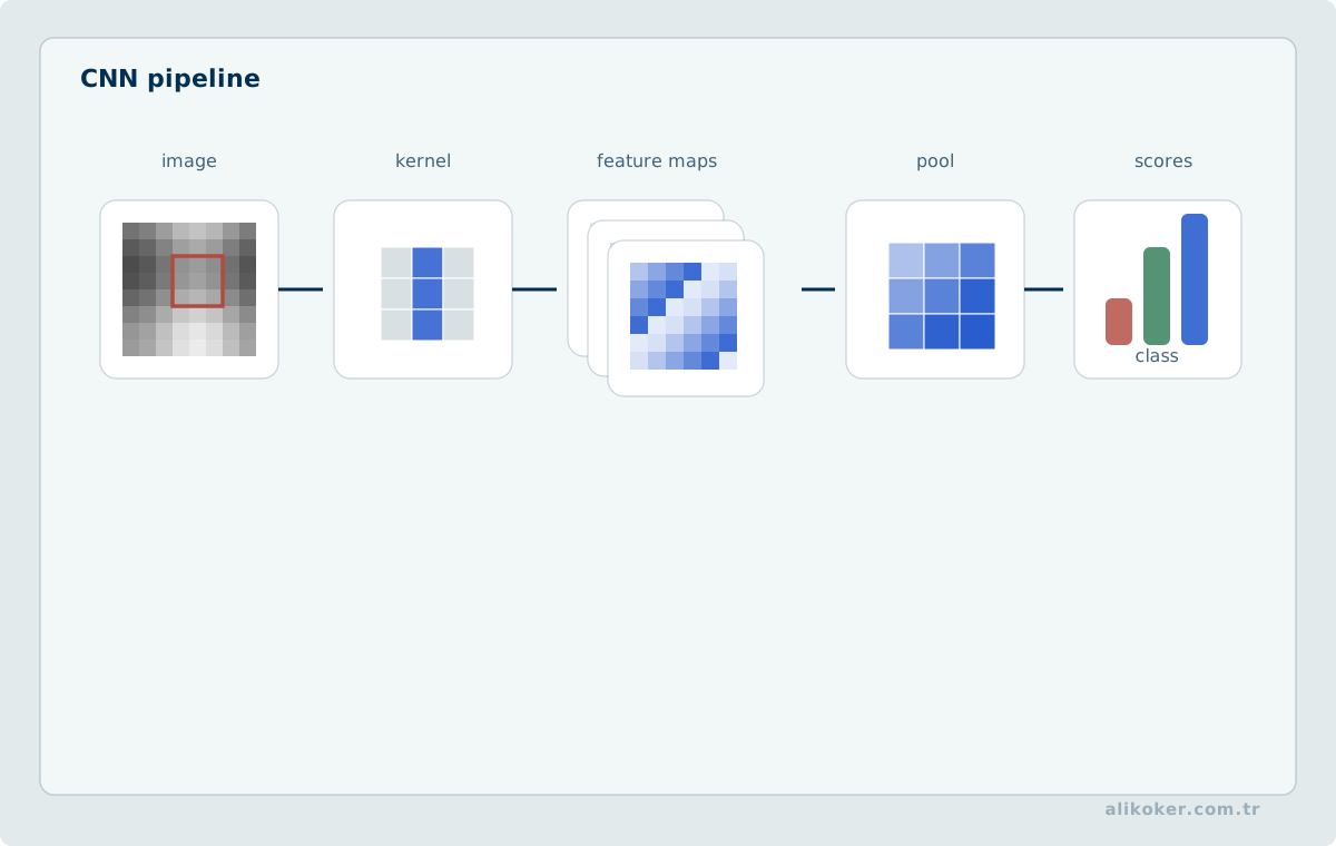
CNN layers also use local weighted operations, but a classical filter kernel is specified by design whereas a learned kernel is fitted from data and an objective. The similarity should not erase the distinction. Classical signal processing keeps physical and spectral assumptions explicit; learned filters expand representation capacity through data.

References

Muhammet Ali Köker; Nursel Yalçın. Görüntü ve Ses İşleme. Nobel Yayınevi, 2022. Source

Yapay Zeka - Kuramdan Uygulamaya. Nobel Akademik Yayıncılık, 2022. Source