Audio Processing and Forensic Audio Engineering

Audio processing concerns the acquisition of mechanical wave motion, its conversion to digital signals, and the analysis of speech and other acoustic events. Forensic audio engineering applies these methods under requirements for measurement validity, preservation of evidence, provenance, error rates, and scientifically defensible interpretation. Improving intelligibility is not equivalent to proving authenticity. Speech recognition, speaker comparison, and source separation also address distinct inference problems.

Audio is a time-dependent physical measurement. Every operation in microphone acquisition, analogue conversion, sampling, encoding, transmission, and processing can influence later estimates. Engineering evaluation must examine not just aggregate task performance but assumptions, robustness to recording conditions, propagation of error, latency, and reproducibility.

Unit 1: Physical and Acoustic Foundations of Sound

Sound is a mechanical pressure disturbance that propagates through a material medium. Digital audio processing begins when a microphone converts that physical variation into an electrical signal and the signal is sampled.

Frequency, amplitude and phase

Frequency describes repetition rate, amplitude describes magnitude, and phase describes relative position within a periodic cycle. Real sounds contain many frequency components. The Fourier transform provides a spectral representation of those components.

Human hearing sensitivity varies with frequency. Perceived loudness is not a linear copy of amplitude, and pitch alone does not determine speaker or source identity.

Wavelength and Propagation

Sound in air is not the transport of air particles from source to listener; it is the propagation of pressure variation through the medium. Particles move only around their equilibrium positions while regions of compression and rarefaction travel.

Frequency f, wavelength λ, and propagation speed c are related by:

c = f · λ

The speed of sound in air depends on temperature and is approximately 343–344 m/s near room temperature. If propagation speed changes at the same frequency, wavelength changes with it.

Low frequencies correspond to longer wavelengths and high frequencies to shorter wavelengths. This relation matters physically in microphone placement, room modes, beamforming, and reverberation.

Propagation and room acoustics

Sound does not propagate in vacuum. Reflection, absorption, diffraction and scattering shape the microphone signal. In enclosed spaces, direct sound combines with early reflections and reverberation. As source-microphone distance grows, the direct-to-reverberant ratio may decrease.

Speech production

Human speech can be approximated with a source-filter model. Excitation from the vocal folds is shaped by resonances of the vocal tract. Formants are particularly important for vowel identity.

The sampling theorem defines the minimum sampling condition for reconstructing a band-limited signal. Real systems use analogue anti-alias filters before digitisation.

A spectrogram is not an image of sound; it is a visual representation of time-varying spectral energy.

Respiration, Larynx, and Vocal Tract

Speech production can be approximated through three physical stages. The lungs supply airflow as the energy source. The larynx produces excitation through vocal-fold vibration or turbulent airflow, and the vocal tract formed by the pharyngeal, oral, and nasal cavities shapes that excitation spectrally.

Not all speech sounds use the same source mechanism. Periodic vocal-fold vibration can dominate vowels, turbulent noise is important in fricatives, and brief transients are important in plosive consonants. Natural speech moves among these source types over time and can combine them.

A phoneme is one of the smallest sound classes that can distinguish meaning in a language. Its acoustic realization changes with speaker, context, and neighboring sounds, so the same phoneme does not produce an identical waveform in every recording. This variability is one of the basic challenges of speech and speaker recognition.

Hearing and Perception

The outer ear collects acoustic energy and directs it toward the eardrum. The ossicles of the middle ear transfer mechanical vibration toward the inner ear. Mechanical and neural transduction in the cochlea plays a central role in encoding frequency content for the auditory system.

Physical sound pressure and perceived loudness are not the same quantity. Likewise, frequency is strongly related to perceived pitch, but hearing does not behave like a linear measuring instrument. Masking, frequency-dependent sensitivity, and temporal context affect perception.

Audio-processing algorithms therefore cannot be evaluated only by numerical signal difference. Codec behavior, denoising, and synthesis should distinguish perceptual change from performance on the downstream task.

Mechanical waves and pressure

Sound travels as fluctuations of pressure and particle velocity around the equilibrium of a material medium. A low-amplitude plane-wave approximation is p(x,t) = A cos(2πft − kx + φ), where frequency is f, wave number is k = 2π/λ, and wavelength is λ. Propagation speed satisfies c = fλ. Sound speed depends on the elastic and density properties of the medium; approximate values for air vary with temperature and composition.

Sound-pressure level is L_p = 20 log₁₀(p_rms/p₀). A decibel expresses a logarithmic ratio relative to a defined reference, not an absolute amplitude without context. Acoustic pressure level and digital full-scale level use different references. Confusing them can invalidate microphone calibration and comparison of recordings.

Propagation, room response, and hearing

Geometric spreading, reflection, absorption, diffraction, and scattering change the time-frequency structure of recorded sound. Early room reflections overlap the direct signal; later reflections form reverberation. Differences in source–microphone distance, orientation, and room impulse response can alter recordings without any change of speaker identity.

Human hearing varies with frequency and level. Perceived loudness does not scale linearly with pressure; pitch and speech intelligibility are separate perceptual attributes. Forensic listening must therefore be supported by measurable acoustic features and reproducible procedures to limit subjective bias.

Room Response and the Physical Reference of a Recording

The microphone signal contains more than the source sound: direct propagation, reflections, ambient noise, and the microphone response are superimposed. An approximately linear time-invariant environment can be represented by y(t) = h(t) * x(t) + n(t), where h(t) describes the impulse response of the room and recording chain. Reverberant delayed copies blur speech boundaries, illustrating why a recorded waveform is not identical to its source.

Microphone distance and orientation, gain, automatic level control, and filters in the recording chain must be documented. A single recording seldom determines the room response and the original source independently. In forensic comparisons, observed spectral variation may arise from speaker properties, room acoustics, or recording hardware; those alternatives must be evaluated. Decibel measurements without an established physical reference can support relative rather than absolute level comparisons.

Unit 2: Digital Audio Representation and Recording

Audio recording begins with a microphone, analogue front end and analogue-to-digital converter. The resulting sample stream can be stored, compressed or transported over a network in real time.

Analog-to-Digital Conversion

A microphone converts variations in air pressure into an electrical signal. The analog front end applies gain and the required filtering, and the analog-to-digital converter samples the signal at discrete times and quantizes each sample to a finite numerical level.

This chain has two distinct forms of resolution:

• time resolution, determined by sampling rate,
• amplitude resolution, determined by bit depth.

Increasing sampling rate does not directly increase quantization resolution, and increasing bit depth does not directly increase temporal resolution. They affect different error mechanisms.

Analog band limiting before conversion is important. If components above the Nyquist frequency are not sufficiently attenuated, sampling can fold them into the baseband as aliasing; this distortion cannot later be removed completely by digital filtering alone.

Sampling and channel layout

Sampling rate defines how many samples are acquired per second. Bit depth affects quantisation resolution and available dynamic range. Channel count may preserve additional spatial or source-separation information.

Blindly reducing multichannel audio to mono can remove useful information for later processing.

PCM and codecs

WAV often carries PCM, but the file extension alone does not guarantee the actual encoding. MP3, AAC and Opus use different lossy coding strategies and introduce different artefacts.

In machine-learning systems, differences in codec, sample rate and channel configuration between training and deployment data can affect model stability.

Real-time transport

Packet duration, loss recovery and jitter-buffer behaviour determine the balance between continuity and latency. Larger buffers absorb network variation while increasing interaction delay.

Clock drift also matters in long recordings. Two devices operating at nominally identical sampling rates may still progress at slightly different effective rates.

Codec, sampling rate, channel layout and timestamps should therefore be treated as part of the audio data contract.

Microphone, sampling, and quantization

A microphone transforms pressure fluctuations into electrical measurements. Analogue gain stages add frequency response, noise, and possible saturation. Without a suitable antialias filter before conversion, frequencies above the sampled bandwidth can fold into the audible range. The ideal sampling theorem assumes band limitation; real filter transition bands and clock uncertainty must also be considered.

Samples can be represented as x[n] = xₐ(n/fₛ). Sampling frequency fₛ determines temporal sampling, while bit depth determines the ideal number of quantization levels. A nominal 16-bit or 24-bit representation does not prove that the physical acquisition chain has equal effective resolution. Dither can reduce structured quantization distortion; the actual noise floor and saturation limits determine practical dynamic range.

Channels, timestamps, and containers

Stereo channels may represent independent acquisition paths, but they cannot always be assigned to different speakers. Microphone placement, cross-talk, mixing, automatic gain, and coding can invalidate such an assumption. Clock drift between multichannel devices creates misalignment. Sample-index time must be distinguished from external wall-clock timestamps.

A container format, sample representation, and compression codec describe different layers. Resampling, mixing, and format conversion may change signal characteristics. The digest of the original file, that of decoded samples, and that of an analysis copy verify different objects; a forensic record must identify the level at which integrity was checked.

Safe Conversion from Recording to Digital Signal

Processing begins by decoding the container and validating codec, channel count, sample rate, sample format, and actual decoded sample count independently. Duration from a header is not assumed correct: the decoded duration is T = N/fₛ. Level normalization changes scale but cannot restore clipped peaks. DC-offset removal and sample-rate conversion are performed on derived copies without modifying the original evidence.

Before downmixing stereo audio, the channels must be classified as separate parties, spatial microphones, or a mixed output. Simple arithmetic averaging can attenuate phase-opposed components and destroy channel provenance. Recording time, channel sample counters, and output offsets require an explicit mapping. Source sample n₀ at rate f₀ occurs at n₀/f₀ seconds and approximately sample round(n₀ f₁/f₀) at target rate f₁; rounding and boundary policies must be consistent across the pipeline.

Unit 3: Time- and Frequency-Domain Audio Analysis

Types of cepstrum

Cepstrum does not denote a single mathematical representation. Several forms are used depending on which spectral quantities are preserved and how the logarithm is defined.

The real cepstrum uses the logarithm of the magnitude spectrum:

c_r[n] = IDFT{log |X[k]|}

Because phase is discarded, the original waveform cannot in general be reconstructed from the real cepstrum alone. The representation is useful for spectral-envelope, periodicity, and echo-related analysis.

The power cepstrum is defined in slightly different ways across texts and libraries, commonly through the squared magnitude of a transformed log spectrum or through a log-power spectrum. Implementations should be compared only after these conventions and their scaling are made explicit.

The complex cepstrum retains magnitude and phase through a complex logarithm:

c_c[n] = IDFT{log X[k]}

Computing the complex logarithm requires phase unwrapping. Using wrapped phase directly introduces discontinuities; an incorrect unwrapping step therefore corrupts the complex cepstrum. Under suitable assumptions, the complex cepstrum is useful in homomorphic analysis and minimum-phase decomposition. It preserves more information than the real cepstrum but is correspondingly more sensitive to implementation details.

Fourier transform, framing, and windows

The discrete Fourier transform is X[k] = Σ(n=0…N−1) x[n] · e^(−j2πkn/N). Frequency sample spacing is Δf = fₛ/N, but this interval does not alone determine the ability to resolve nearby sinusoids. Effective frequency resolution depends on observation duration and the window's main lobe. When a segment is not periodic at its boundaries, spectral leakage occurs. Window selection trades main-lobe width against sidelobe rejection.

The short-time Fourier transform X(m,k) = Σₙ x[n] · w[n−mH] · e^(−j2πkn/N) reveals a changing spectrum. A short window improves timing of transient events while limiting low-frequency discrimination; a long window reverses this compromise. Hop size H controls overlap and computational cost. Analysis and synthesis windows must satisfy appropriate overlap-add reconstruction conditions when the signal is reconstructed.

Spectral measures and cepstrum

Magnitude spectra, power spectra, and power spectral density have different physical and statistical meanings. The real cepstrum, obtained from an inverse transform of log spectral magnitude, helps examine multiplicative source–filter behaviour in an additive representation. Numerical protection is needed near zero-valued spectral bins. Mel-frequency cepstral processing introduces a filter bank, logarithm, and cosine transformation; the choices of scale, spacing, and normalization are consequential. Spectrogram colour intensities should not be compared across recordings without a common scaling convention.

Discrete frequency spacing and temporal resolution

At a sampling rate of fₛ = 16000 Hz, a frame with N = 400 samples lasts 25 ms. The DFT sample spacing is 16000/400 = 40 Hz. Zero-padding this frame to 512 transform points makes the displayed spectrum denser, but does not extend the observation interval or improve physical resolving power to the same degree. A hop of H = 160 samples corresponds to 10 ms steps and 60% overlap.

A bright spectrogram component does not, by itself, establish speaker identity or sound-source class. Window normalization, magnitude versus power display, logarithmic scaling, and channel gain affect plotted values. Quantitative comparison requires consistent windows, spectral normalization, and reference levels.

Reconstruction from Overlapping Windows

The short-time Fourier transform depends on analysis window, frame length, and hop size. An incorrect inverse-window convention produces artificial time-varying gain. After inverse transforms, overlapping synthesis frames are accumulated with normalization derived from the analysis and synthesis window products: y[n] = Σₘ wₐ[n−mH]wₛ[n−mH] x[n] / Σₘ wₐ[n−mH]wₛ[n−mH], evaluated where the denominator is nonzero. Boundary frames require explicit padding and truncation rules.

Overlap alone does not guarantee exact reconstruction; window family and synthesis weights matter. Algorithmic latency includes the samples needed to form the analysis window and any additional look-ahead. More overlap can increase computation and buffering in live processing. A spectral enhancement implementation should first demonstrate sample-level reconstruction under a unit gain mask, before evaluating its behaviour with a nontrivial noise-suppression mask.

Unit 4: Speech Production Models and Features

Mathematical Structure of the MFCC Pipeline

An MFCC vector is usually calculated from overlapping short-time frames. Pre-emphasis, window type, frame length, use of a power or magnitude spectrum, filter count, Mel conversion formula, cosine-transform normalization, and treatment of the energy coefficient vary between implementations. MFCC is not one immutable standard vector. It is a family of implementations that follow the same design principle.

Let P_t[k] be the power spectrum obtained from the discrete Fourier transform of frame t. The output of Mel filter m can be written as:

E_t[m] = Σ_k H_m[k] P_t[k]

H_m[k] is commonly a triangular weighting function that overlaps adjacent filters. Filter centers are not equally spaced on the linear Hertz axis. They are placed at roughly equal intervals on a Mel axis. One frequently used mapping is:

mel(f) = 2595 log10(1 + f / 700)

This is not the only valid definition of the Mel scale. Other sources use equivalent natural-log forms, different constants, or piecewise linear-logarithmic mappings. The original Davis and Mermelstein arrangement also used linear spacing at low frequencies and logarithmic spacing at higher frequencies. Seemingly small differences between implementations can produce numerical differences, especially when low-frequency filters are mapped onto discrete Fourier bins.

A logarithm is applied to the filter outputs:

L_t[m] = log(E_t[m] + ε)

The positive floor ε prevents an undefined logarithm at zero energy. The logarithm serves two purposes. It compresses the wide dynamic range of spectral energy, and it turns the multiplicative interaction of source and filter in the frequency domain into an approximately additive structure. The second property is the main connection between cepstral representation and the speech production model.

The final stage usually applies a type-II discrete cosine transform to the log filter-bank vector:

c_t[r] = Σ_(m=0)^(M-1) L_t[m] cos[πr(m + 1/2) / M]

M is the number of filters, r the cepstral order, and c_t[r] the corresponding MFCC component. Lower-order coefficients carry the broad slope and envelope of the Mel spectrum. Higher orders describe faster variation across filters. Most pipelines retain only an initial subset. This truncation is not merely dimensionality reduction. It deliberately applies a low-pass operation to spectral detail.

The discrete cosine transform also tends to reduce correlation between log filter energies. Adjacent Mel bands are strongly related because the triangular filters overlap. The transform maps this correlated vector into coefficients that are more nearly separated. This property was especially important for Gaussian mixture models using diagonal covariance assumptions.

Losing the Right Information

One of the defining properties of MFCC is that it is not a high-fidelity audio representation. It discards phase, smooths harmonic structure, suppresses fine spectral detail, and often normalizes absolute energy. These losses can be severe for coding or resynthesis, but they are useful in many recognition tasks.

A speech recognizer does not need to reproduce the microphone waveform. It needs examples of the same phonetic unit, recorded with different pitch, phase, level, and channel conditions, to occupy a reasonably compact region of feature space. MFCC does not remove all unwanted variation, but it moves the representation in that direction. The value of a feature vector is therefore determined less by the total information it contains than by the ratio between task-relevant discrimination and irrelevant variability.

The Mel filter bank allocates more resolution to low frequencies. Since the first formants and many important spectral transitions occur there, a fixed number of features can be used more effectively than with uniform linear-frequency sampling. Wider bands at high frequencies reduce the influence of narrow and unstable spectral changes. Davis and Mermelstein also associated MFCC's advantage over a linear-frequency cepstrum with its stronger suppression of less relevant high-frequency variation.

The statement that the Mel scale imitates the human ear is still an overgeneralization. MFCC does not fully model equal-loudness contours, auditory masking, temporal masking, cochlear nonlinearities, or neural coding. It uses a psychoacoustically inspired frequency resolution. It is not a biophysical model of hearing.

No fixed phonetic meaning can be assigned to each MFCC coefficient either. The first coefficient can relate to overall spectral level or slope, and later coefficients to finer envelope shapes, but they cannot be interpreted directly as the first formant, second formant, or a particular phoneme. Because every DCT basis vector spans the entire filter bank, each coefficient expresses the weight of a global spectral pattern.

Why MFCC Fit Classical Recognizers

MFCC succeeded for engineering reasons as well as perceptual ones. Its structure matched the computational and statistical assumptions of classical speech recognition systems.

The processing cost is low and predictable. Each frame requires a fast Fourier transform, multiplication by a sparse filter bank, a logarithm, and a small cosine transform. The approximate cost is O(N log N) for the Fourier transform, additional work proportional to the nonzero filter weights, and a small matrix-vector multiplication. Filter and DCT coefficients can be precomputed. The pipeline can run in streaming form with fixed memory and deterministic work per frame.

The output is compact. A few dozen coefficients replace hundreds of Fourier magnitudes. This reduced both storage and distance-computation cost in systems based on dynamic time warping, hidden Markov models, and Gaussian mixture models. The original Davis and Mermelstein experiment also reported compact representation with few coefficients as one of the method's advantages.

Cepstral space is suitable for simple distance measures. The DCT's approximate decorrelation makes inexpensive methods such as Euclidean distance and diagonal-covariance probabilistic models more practical. The original comparison used Euclidean distance for cepstral features, and MFCC performed well under that simple metric.

The pipeline also accepts normalization naturally. Cepstral mean subtraction, variance normalization, and first- or second-order temporal derivatives can be added without changing its basic structure. Mean subtraction can reduce part of a fixed channel response, while derivative coefficients add short-term motion to an otherwise static frame vector. Typical front ends in the early 2000s used MFCCs together with mean and variance normalization, temporal derivatives, and linear discriminant transforms.

The method is independent of the downstream model. The same MFCC extractor can feed template matching, HMM-GMM systems, support vector machines, or neural networks. This separation allows the feature stage to be verified independently, reproduced on different platforms, and monitored more easily in production.

The cost of these advantages is a fixed information bottleneck. Phase, fine harmonic structure, and high-resolution spectral detail discarded by the extractor cannot be recovered by the later model. Noise and channel distortion are mixed into filter energies before the logarithm, so MFCC is not inherently noise invariant. Normalization can reduce some mismatch, but it does not guarantee robustness at low signal-to-noise ratios or under strong reverberation.

MFCC in the Deep Learning Era

End-to-end and self-supervised speech models removed the requirement for hand-designed low-dimensional features. Systems such as wav2vec 2.0 and HuBERT feed raw waveforms into convolutional front ends and learn a representation from data. They are not constrained by the bottleneck fixed in advance by MFCC.

Not every modern system operates directly on the waveform. speech recognition model uses a log-Mel spectrogram rather than MFCC. The distinction matters. A log-Mel spectrogram retains the Mel filter bank and logarithmic compression but does not apply DCT-based cepstral compression. The network can observe local structure between Mel bands and learn which spectral combinations are useful.

These developments do not remove MFCC's historical value. They change the conditions under which it is a rational choice. Learned waveform features or log-Mel representations can be preferable when large data sets, high compute budgets, and end-to-end optimization are available. MFCC remains useful when systems require fixed latency, limited memory, low power consumption, transparent preprocessing, small training sets, or bit-level reproducibility.

MFCC persists not because it models hearing perfectly or provides the highest accuracy for every speech problem. It combines the physical signal, perceptual frequency resolution, statistical modeling, and computation cost in a balanced information bottleneck. Its broader lesson for system design is straightforward: the best representation is not the one that preserves every detail of the input, but the one that retains the structure required by the target task with the least irrelevant variability and cost.

Audio features transform raw waveforms into representations that are more stable for matching, classification and recognition. Depending on the task, systems may use time-domain features, spectral representations or learned embeddings.

Preprocessing: Pre-emphasis, Framing, and Windowing

Classical speech-processing pipelines do not usually analyze a long recording as one block. Speech is treated as approximately stationary over short intervals, so the signal is divided into frames that are analyzed separately.

Pre-emphasis was historically used to increase the relative contribution of higher-frequency components. A simple form is:

y[n] = x[n] - α x[n-1]

where α is selected for the application. Pre-emphasis is not mandatory for every modern model; matching the preprocessing used during training is more important, especially for systems that consume raw waveforms or log-Mel features.

Cutting frames with hard boundaries can increase spectral leakage. Hamming and related windows taper frame edges. Window length and frame shift determine the balance between temporal and frequency resolution.

The FFT provides an efficient way to decompose a windowed frame into frequency components. Repeating this calculation over successive frames produces the STFT time-frequency representation. Filter banks, MFCCs, and later cepstral processing can then operate on this short-time spectral structure.

Time and frequency features

Short-time energy and zero-crossing rate are inexpensive time-domain measures. STFT computes frequency components within short windows and produces a time-frequency representation. Window length creates a direct trade-off between temporal and frequency resolution.

MFCC and spectral representations

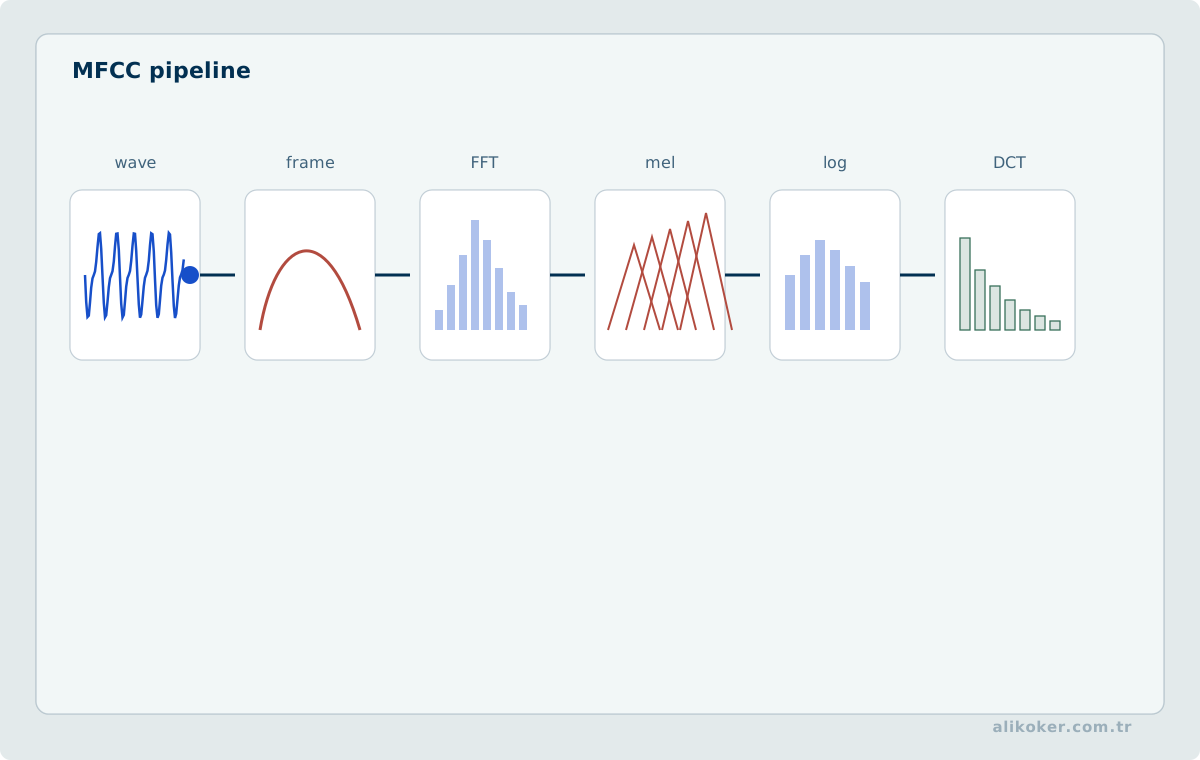
MFCC is derived from log Mel-filterbank energies followed by a cepstral transform. It has long been a standard feature for speech recognition and speaker modelling.

Pitch, formants, spectral slope, jitter and shimmer represent different physical or perceptual properties of the signal.

The Computation Chain for Speech Features

An acoustic classifier requires fixed conventions for channels and sample rates; clipped or nonspeech frames are marked before feature extraction. If pre-emphasis is used, its coefficient and frequency response must be specified, rather than assuming it benefits every learned representation. Framing and windowing precede power-spectrum estimation, filter-bank integration, logarithmic compression, and optional cepstral projection. An energy floor preventing log(0) also affects the distribution of low-energy frames.

Normalization statistics computed on the training set are not re-estimated using test data. Utterance-level normalization can discard different information from recording-level or speaker-level normalization; the appropriate invariance depends on the task. Changing denoising, VAD, and feature extraction simultaneously prevents attribution of a gain or regression to any particular stage. Controlled experiments should vary one decision at a time while holding test splits and scoring rules fixed.

Learned embeddings

Modern systems can map an audio segment directly to a dense speaker embedding or a more general audio embedding. Matching can use cosine similarity, PLDA or learned scoring models.

Channel, microphone, codec and acoustic environment can change the representation distribution, so normalisation and domain adaptation belong in the feature pipeline.

At scale, vector dimension also determines storage cost, index size and query latency.

Source–filter representation

Voiced speech can be approximated as an excitation shaped by the resonances of the vocal tract. In a local linear model, S(z) = E(z)H(z). Formant regions can provide information about vocal-tract resonances, whereas fundamental frequency describes excitation periodicity; they are not equivalent. Articulation, recording channel, anatomy, and speaking task affect formant estimates.

Linear prediction approximates speech by x[n] ≈ −Σ(k=1…p) aₖx[n−k] + e[n]. Model order matters: an underspecified model can merge resonances, while excessive order may create spurious peaks. Cepstral liftering approximately separates slowly varying spectral envelopes from finer excitation structure, but does not provide a physically exact decomposition in all conditions.

Classical and learned representations

Frame energy, zero-crossing rate, pitch, spectral centroid, and spectral slope characterize different aspects of acoustic observations. Mel-frequency cepstral coefficients are obtained from transformed log filter-bank energies. Window duration, number of coefficients, pre-emphasis, normalization, and derivative features affect the result. The cepstrum is a broader mathematical concept than a particular Mel-feature extraction pipeline.

Learned acoustic embeddings can represent higher-level patterns for classification or sequence processing. Their utility depends on training objectives, recording duration, language, and domain shift. A representation optimized for speaker comparison is not necessarily suitable for emotion analysis or acoustic-event classification.

Unit 5: Noise Reduction and Audio Enhancement

Audio restoration estimates a cleaner or more task-useful signal from degraded recordings. Noise, reverberation, clipping and packet loss represent different degradation models.

Noise Type and Filter Selection

Noise is not one class of disturbance. Approximately stationary background hum, narrowband mains interference, broadband noise, impulsive corruption, wind, mechanical vibration, and competing speech have different temporal and spectral structures. A “noise filter” should therefore not be treated as one universal operation.

Classical filters serve different frequency-domain purposes:

• a low-pass filter attenuates higher frequencies,
• a high-pass filter attenuates lower frequencies,
• a band-pass filter preserves a selected interval,
• a band-stop or notch filter suppresses a selected interval.

Cutoff frequency is not a fixed recipe. The useful speech spectrum, recording device, sampling rate, and location of the interference should be considered together. A poorly selected filter can remove speech information along with the noise.

Periodic or narrowband interference may have a clear spectral signature, whereas changing environmental noise can defeat a fixed filter. Noise estimation, adaptive methods, or learned models may then be required.

Noise reduction

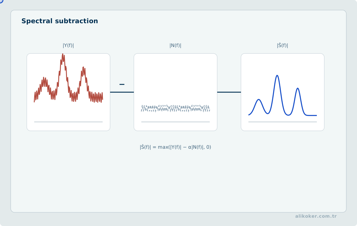
Spectral subtraction and Wiener filtering can suppress stationary or slowly varying noise when noise statistics are estimated reliably. Poor estimates may introduce musical-noise artefacts.

Learned denoisers can handle more complex noise but may also suppress signal components outside the training distribution.

Echo and microphone arrays

Acoustic echo cancellation adaptively models the path from loudspeaker to microphone. Multi-microphone beamforming uses phase and delay differences to reinforce sound arriving from selected directions.

Packet-loss concealment estimates missing samples, while declipping attempts to reconstruct saturated regions.

Task-oriented evaluation

Perceptual improvement does not always improve downstream models. In ASR, speaker recognition or acoustic-event detection, enhancement should be evaluated together with task metrics.

For forensic use, the original recording remains separate, while filter parameters, software version and derived copies are preserved as part of the processing chain.

Boundary of Forensic Audio Enhancement

In forensic audio, the objective is not merely to make a recording sound better; it is to improve examinability while preserving the original evidence. Hum or narrowband interference that masks speech can be reduced, but every filter also changes some part of the signal.

A spectrogram is useful because it shows time, frequency, and energy together, helping distinguish speech structure, interference, and recording artifacts. A single spectrogram, however, is not a deterministic “voiceprint” that proves speaker identity. Speaker comparison must be interpreted together with recording conditions, method, error rates, and uncertainty.

A defensible processing chain preserves the original file as read-only evidence and produces a separate working or derived copy. Recording filter choice, parameters, software version, input/output hashes, and processing order makes the result reproducible and auditable.

Noise estimation and spectral filtering

The additive model y[n] = s[n] + v[n] separates target signal and noise; reverberation or channel distortion requires a more general convolutional model. Stationary background noise and short impulses require different estimators. Spectral subtraction attenuates an estimated noise spectrum but can generate musical noise or remove weak speech harmonics. Wiener filtering derives a gain from expected signal and noise power and depends on reliable statistical estimation.

Adaptive filters update coefficients from an error signal. An excessively large adaptation step may cause instability, whereas an overly small step responds slowly to changing acoustic conditions. Spatial filtering combines microphone channels according to assumed source direction; a direction mismatch can suppress the desired speaker.

Noise Profiles, Gain Estimation, and Auditory Artifacts

Noise suppression first requires determining whether an interval labelled silent actually contains only background noise. A profile contaminated by speech can cause the target speech to be suppressed. Under an approximate uncorrelated stationary-noise model, spectral powers can be written Pᵧ = Pₛ + Pₙ; the assumptions do not hold universally. A minimum-mean-square-error spectral gain can be written G(k,m) ≈ Pₛ(k,m)/(Pₛ(k,m)+Pₙ(k,m)), so overestimating noise power may remove speech components. A soft mask can reduce the musical-noise artifacts associated with hard spectral zeroing.

Competing algorithms must be applied to identical test recordings with consistent sample rates, gain conventions, and time alignment. When clean references are available, signal-distortion measures can be combined with independent recognition error and listening assessments. Improving SNR does not necessarily reduce word error. In forensic processing, the original, intermediate signals, and complete filter parameters remain separate. Enhanced intelligibility is not evidence that previously absent phonetic detail has been recovered reliably.

Limits of evidential enhancement

Learned enhancement can produce more intelligible output while also generating speech-like features favoured by its training distribution. Such generated detail was not directly measured in the source recording. Enhanced media must not replace the original. Controlled listening, artifact inspection, and task-based evaluation are needed to assess the effect of processing.

SNR is meaningful when reference signal and noise components are known, as in controlled experiments. In forensic recordings they usually are not. No-reference quality measures also do not prove evidential accuracy. A filter's effect on intelligibility can be tested with independent listening or suitably annotated evaluation data.

Unit 6: Multichannel Audio and Spatial Processing

Channel ownership and VAD decisions

The reliability of channel ownership depends on the following infrastructure assumption:

channelOwner(left) = A
channelOwner(right) = B

This mapping can be provided in structures such as two-party telephone, radio, or operator systems. However, the presence of energy in a channel does not by itself establish that the channel owner is speaking. Cross-channel leakage, speaker-microphone echo, automatic gain control, environmental noise, tones, short impulses, and codec artifacts can create false activity.

For this reason, the following energy comparison is insufficient:

energy(left) > energy(right) then speaker A

This rule only selects the dominant amplitude. It does not determine speech activity, whether the other channel is truly silent, or whether both channels carry speech simultaneously. A more robust approach produces an independent VAD decision for each channel:

VL = 0, VR = 0 → silence
VL = 1, VR = 0 → left-channel candidate
VL = 0, VR = 1 → right-channel candidate
VL = 1, VR = 1 → simultaneous or ambiguous activity

There is no universally correct policy for simultaneous activity in both channels. Under a single-active-segment and non-overlapping-output constraint, preserving the priority of the current owner is a deterministic choice. When the active segment belongs to A and both channels become active, A continues; B can become the owner only after A activity ends and B activity is confirmed. This approach does not represent every detail of genuine simultaneous speech, but it does not produce overlapping time intervals and is compatible with downstream ASR systems that expect a single audio stream.

Time differences and source direction

The arrival-time difference Δt between two microphones depends on geometry and incident direction. Under suitable far-field plane-wave assumptions, Δt ≈ d sin(θ)/c; the angular convention must be stated. Correlation and phase-based estimators can measure delay. Reflections and multiple sources create competing peaks, so a single delay estimate is not necessarily correct.

Beamforming delays and weights channels to emphasize selected directions. Narrowband and broadband settings require different designs. A spatial filter that improves intelligibility does not by itself establish source location as forensic fact; array calibration and geometric uncertainty remain relevant.

Separating Channel Leakage from Spatial Delay

A level difference between channels does not independently establish speaker ownership. Comparable sampling clocks and channel delays must first be confirmed. A peak in cross-correlation may estimate relative delay of a common component, but reflections, automatic gain, and simultaneous sources create ambiguity. Leakage of speech between channels can generate similar waveforms with a consistent lag and should not be mistaken for a second independent speaker.

Per-channel VAD decisions are aligned to one sample timeline. When an acquisition contract assigns channels to parties, inferring their identities again from voice similarity is unnecessary; leakage suppression or an uncertainty state is more appropriate. Without such metadata, direction estimates are meaningful only under an explicit microphone geometry and acoustic model. Under the two-microphone far-field approximation, the physically plausible delay satisfies |Δt| ≤ d/c; larger estimates warrant investigation of synchronization, geometry, or multipath interference.

Physical channels versus identity

Where the recording configuration has been verified, independent channels can strongly assist speaker separation. In mixed recordings or shared acoustic spaces, channel identity need not equal speaker identity. Channel assignment, timestamps, and voice activity can be combined while overlapping speech receives separate treatment. Deterministic speaker labels are valid only if deterministic ownership is a real property of the recording chain.

Unit 7: Audio Segmentation and Voice Activity

Frame, turn, and segment durations

VAD operates on short PCM frames. In the example configuration, the sampling rate is 16 kHz, the sample format is 16-bit signed little-endian, and the frame duration is 10 ms. The number of samples in a single-channel frame is:

N = 16000 × 0.010 = 160 samples

With two bytes per sample, the mono frame size is 320 bytes and the stereo interleaved frame size is 640 bytes:

160 × 2 = 320 bytes
160 × 2 channels × 2 bytes = 640 bytes

A single 10 ms VAD decision should not be converted directly into a segment-opening or speaker-switching decision. Noise impulses, plosive consonants, echo, and transient leakage can cause short-lived decision changes. Three time scales should therefore be separated:

1. Frame level: the instantaneous VAD observation.
2. Turn level: the short window in which a speaker change is confirmed.
3. Segment level: the longer time interval sent to ASR or another model.

The active owner is not changed until a candidate owner remains dominant for a specified number of consecutive frames:

candidateFrames >= confirmThreshold

With 10 ms frames, confirmThreshold = 4 corresponds to an approximately 40 ms confirmation window. Eight frames provide an approximately 80 ms observation. These thresholds do not measure a linguistic unit. They test the temporal stability of the signal decision.

A state machine with one active segment can be established using the following variables:

owner ∈ {NONE, A, B}
segmentStart
segmentEnd
candidateOwner ∈ {NONE, A, B}
candidateCount
silenceCount

When there is no active owner and only one channel carries speech for a sufficient duration, a new segment is opened. When A is active and the left channel remains active, the segment is extended. When the left channel becomes silent and the right channel becomes active, a direct A → B transition is not performed; B first becomes a candidate. If the confirmation period is completed, the A segment is closed and a B segment is opened:

A → candidate B → B

Silence and duration limits

Silence tolerance can vary according to segment length:

segment < 3 seconds → approximately 1000 ms
3 seconds ≤ segment < 25 → approximately 300 ms
segment ≥ 25 seconds → approximately 200 ms

The piecewise threshold function is:

 1000 ms, 0 ≤ T < 3
G(T) = 300 ms, 3 ≤ T < 25
 200 ms, T ≥ 25

Here, T is the active segment duration and G(T) is the consecutive silence duration required to close the segment. A longer wait for short segments prevents a natural pause after one or two initial words from closing a segment prematurely. A shorter threshold for long segments limits segment growth, model-call latency, and memory use.

Two distinct duration limits can be used together:

target duration : 25 seconds
hard upper limit: 29 seconds

The application behavior is defined as follows:

T < 25 s
 apply natural silence rules

25 s ≤ T < 29 s
 close at the first suitable silence

T ≥ 29 s
 force closure without waiting for silence

The target duration favors closure at natural pauses. The hard upper limit strictly bounds segment size during uninterrupted speech. These limits help control ASR inference time, temporary tensor sizes, feature-extraction cost, queue latency, and the volume of data to be reprocessed after an error.

The hard limit should be aligned to a frame boundary. With 10 ms frames, 29 seconds equals 2900 frames:

29 × 100 = 2900 frames

To avoid rounding errors, duration can be tracked using processed sample or frame counts rather than floating-point seconds:

frameStart = processedSamples
frameEnd = frameStart + validSamples

The timestamp is derived from sample position:

timeMs = sampleIndex × 1000 / sampleRate

For 16 kHz:

timeMs = sampleIndex / 16

The integer-division order and rounding policy must remain the same throughout the system.

Minimum speech duration

Sending every VAD activity directly to the model is inefficient. Short noises, interjections, and partial words can generate unnecessary inference. Two separate lower limits can therefore be used:

minimum actual speech duration : 1 second
minimum model input duration : 3 seconds

Activity shorter than one second can be rejected as a segment. Valid speech between one and three seconds can be extended to three seconds with silence before it is sent to the model. Validity and model-input size should be evaluated using separate variables:

speechDuration = actual active speech duration
modelDuration = speech + added silence

The validity decision should be based on speechDuration, whereas the model input size should be based on modelDuration. Padding does not increase content; it only satisfies the model's minimum input requirement.

For mono input, one VAD result can be routed directly to a general speaker label or to A:

V(t) = 1 → A
V(t) = 0 → NONE

For stereo input, channels are separated into distinct buffers and independent VAD is applied. Both input types can pass the same information to a shared route mechanism:

owner
PCM data
valid byte count
frameStart
frameEnd

The segmentation infrastructure therefore remains shared; only the ownership-determination stage differs:

mono → one VAD result
stereo → two VAD results + ownership policy

The interleaved stereo PCM layout is L0, R0, L1, R1, L2, R2, .... When channels are copied to separate buffers, sample number n in both channels must represent the same time position. The processed sample count should represent the time axis per channel:

processedSamples += validSamplesPerChannel

The total stereo sample count or total byte count should not be added directly to this variable.

Audio segmentation divides a continuous audio stream into meaningful time intervals such as speech, silence, speaker changes or acoustic events. Segment boundaries directly determine the input distribution seen by downstream recognition and classification models.

Voice activity detection

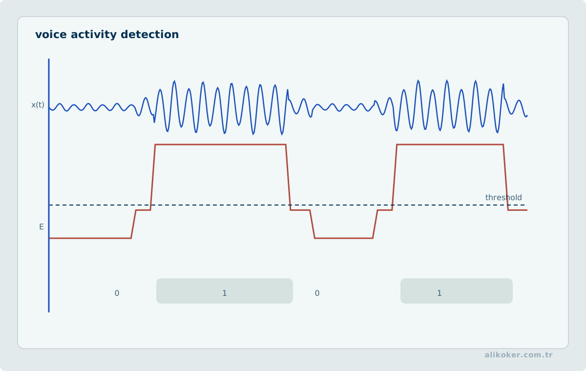
Voice Activity Detection estimates whether speech is present in short time intervals. Energy-based methods are inexpensive, while learned models are generally more robust under variable noise.

Frame-level decisions are stabilised with temporal parameters such as minimum speech duration, silence tolerance and hangover.

Speaker and event boundaries

Speaker changes can be detected from differences between neighbouring acoustic representations. In a speaker diarization pipeline, segments are converted to embeddings and clustered. Overlapping speech allows multiple speakers to be active in the same interval.

Acoustic-event segmentation requires both class and boundary timing to be correct. Event-based F1 and timing tolerance may therefore be more informative than frame accuracy.

System effects

Frame size, overlap and buffering determine latency and computational cost. Very short segments may not provide enough context to ASR or speaker models, while very long segments can merge unrelated events.

Segmentation is therefore a core system layer rather than a minor preprocessing step.

Framing and detection decisions

Frames support classification from energy, spectral changes, or speech-specific statistics. Short windows can localize boundaries accurately but increase decision variance. Longer windows average short fluctuations while adding onset latency. Voice activity detection and speaker-turn detection are different tasks: continuous speech does not imply an unchanged speaker.

Different start and end thresholds, minimum speech length, silence duration, and confirmation intervals may prevent rapid switching between speech and nonspeech. Every confirmation interval contributes latency. A binary speech mask alone cannot describe the number of simultaneous speakers during overlap.

From Voice Activity Decisions to Segments

A frame-wise VAD probability series is not itself a segment list. A state machine with distinct entry and continuation thresholds can reduce rapid toggling near the decision boundary. A bounded hold interval may preserve short inter-word silences without indiscriminately merging successive speakers. Context padding is computed from source-sample offsets; segment durations must not be accumulated from independently rounded millisecond values.

If a downstream model accepts at most L samples, longer speech intervals must be divided. Choosing low-energy regions can reduce, but cannot eliminate, the risk of splitting words. The trade-off between dropping short intervals, merging them, and processing them separately must be measured. Evaluation extends beyond frame accuracy to missed speech duration, extra nonspeech time, boundary damage, segment count, end-to-end latency, and ASR error. Every timing transformation must retain the original sample counter as its reference.

Boundary errors and downstream effects

Truncating the beginning or end of a word may create errors unrecoverable by later speech recognition. Long segments preserve context but increase memory and first-result latency; short segments may split words. Forensic segments must retain precise source-recording time ranges. Decoder priming delays and resampling-induced clock offsets require explicit accounting.

Unit 8: Speaker Recognition and Diarization

Limits of determinism

When fixed frame sizes, preallocated buffers, integer sample counters, and explicit state transitions are used, processing cost per frame remains approximately constant:

O(N)

Here, N is the number of samples in a frame. Total cost grows linearly with audio duration:

O(F × N)

F denotes the total number of frames. Creating new objects, collections, streams, lambdas, or temporary channel arrays for every frame can increase garbage-collector pressure and latency variability. Preallocated buffers and reused VAD states make temporal behavior more predictable. Producing the same segments from the same input allows VAD, channel selection, ASR, and text post-processing to be examined separately during debugging.

Channel-based ownership is not a method that can replace general diarization in every case. Channel identity cannot be used as speaker identity when multiple people use the same channel, microphones are not fixed to speakers, stereo recording is created only for spatial audio, channels are mixed, one speaker is distributed similarly across both channels, or routing changes between recordings. Under these conditions, methods such as embedding-based representations, clustering, speaker verification, or beamforming are required.

Conversely, when channel mapping is reliably supplied by the infrastructure, re-estimating speaker identity can add unnecessary computation and uncertainty. VAD observes only speech activity; channel mapping provides identity; the state machine provides temporal consistency; and segmentation rules preserve the latency and input limits of the downstream model.

Validity Condition for Deterministic Information

The crucial precondition is that channel identity truly encodes speaker role. If the acquisition contract fixes channel 0 as one side and channel 1 as the other, speaker identity is metadata known before inference; estimating the same mapping again with a diarization model can add avoidable error. If stereo instead means two microphones or spatial channels and person-to-channel assignment can change, the deduction is invalid.

Speaker recognition produces identity-related similarity scores from speech samples. Identification, verification and diarization are different decision problems.

Identification and Verification

Speaker recognition contains two different decision problems.

Speaker verification tests a claimed identity. A test recording is typically compared with one enrolled speaker model, asking whether the recording belongs to the claimed person.

Speaker identification searches for which known speaker best matches the recording. The test sample is compared with multiple candidates, and an open-set system can return “unknown speaker” if no candidate reaches a sufficient score.

Both tasks can share the same embedding infrastructure, but candidate population, threshold calibration, and error costs differ. A verification threshold should not automatically be assumed to be suitable for multi-candidate identification.

Text-Dependent and Text-Independent Recognition

A text-dependent system expects a particular word, passphrase, or utterance during enrollment and testing. The system can use both speaker characteristics and consistency with the expected content, which is useful in controlled access scenarios.

A text-independent system does not know in advance which words the speaker will say. The model attempts to extract speaker-related characteristics that remain useful across changing phonetic content. This is more appropriate for free speech, telephone conversations, or archival recordings where the linguistic content is not controlled.

Text dependence is not the same problem as speech recognition. Automatic speech recognition can verify whether the expected phrase was spoken, while the speaker model separately scores how well the voice characteristics match the enrolled person.

Classical approaches

GMM-UBM systems compare a speaker distribution with a universal background model. The i-vector approach represents speech in a compact total-variability space. Methods such as PLDA score similarity between these representations.

Learned representations

Modern systems use x-vectors and related speaker embeddings. Training encourages samples from the same speaker to be close while separating different speakers.

Speaker recognition converts a continuous score into accept or reject decisions using a threshold. Channel mismatch, codec, utterance duration and background noise can shift score distributions.

Speaker diarization

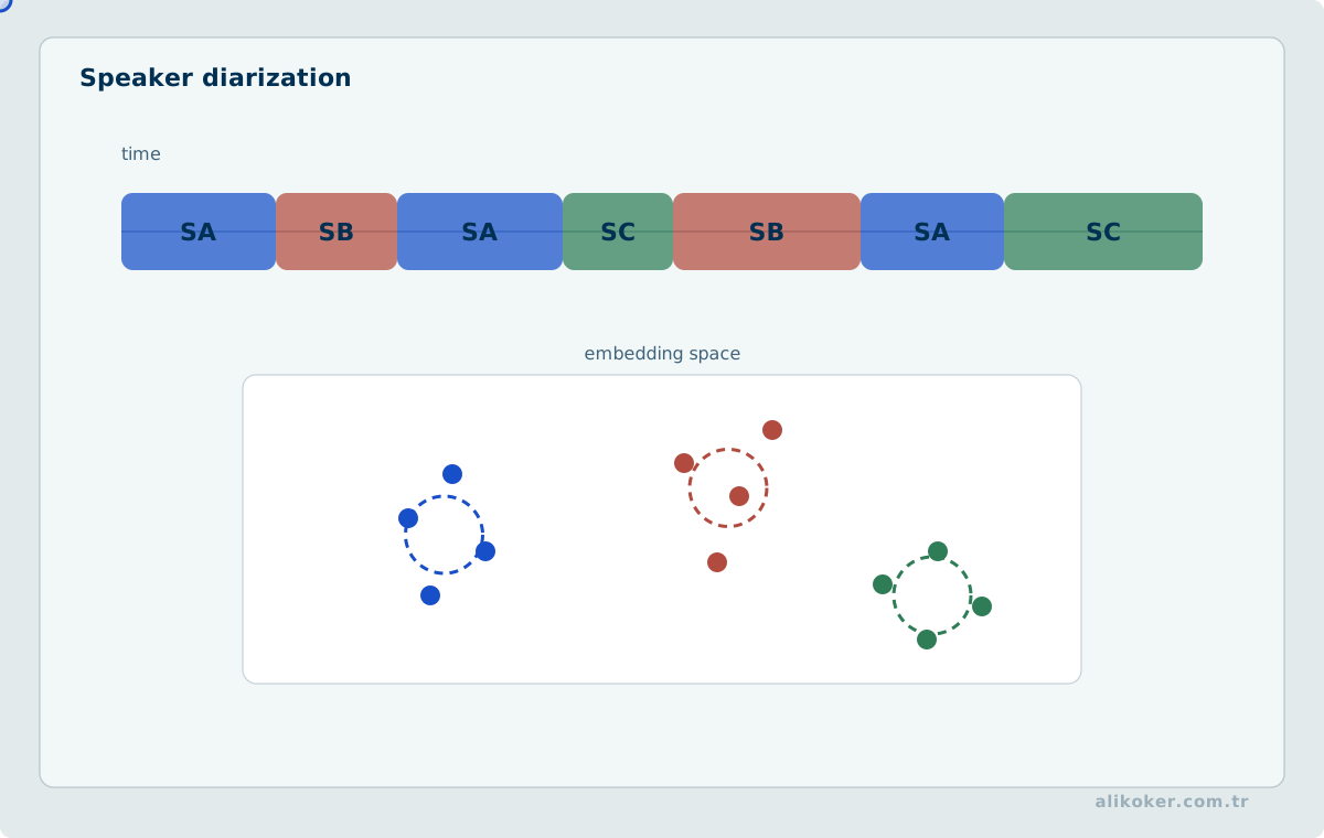
Speaker diarization answers “who spoke when?” by combining VAD, segment embeddings and clustering. Unknown speaker count and overlapping speech remain difficult conditions.

A speaker score is not a deterministic identity marker; it should be interpreted together with threshold calibration, recording conditions and measured error rates.

Embeddings, Clustering, and Uncertainty in Diarization

When channel identity is not provided, diarization begins with speech interval detection. Speaker embeddings are extracted from segments of adequate duration and acoustic variety; very short segments yield unstable representations. Embeddings are compared under consistent models and normalization, and thresholds are selected using development recordings. When speaker count is unknown, clustering requires a model-selection and uncertainty policy. Adjacent segments are not automatically assigned one identity merely because they occur close in time; context can regularize brief ambiguities when supporting evidence is present.

Overlapping speech cannot be faithfully represented by forcing a single speaker label at every instant. Systems restricted to single-label timelines must document this loss. Error analysis distinguishes activity detection, boundary placement, clustering, and overlap errors. The costs of opening a spurious new speaker cluster and merging distinct speakers may differ by application. Automated diarization labels are not proof of forensic speaker identity.

Distinct inference tasks

Speaker identification selects among identities; verification tests a claimed identity; diarization labels when different speakers are active. If diarization produces anonymous speaker clusters, associating those clusters with actual identities requires an additional identification step. Source separation estimates individual acoustic sources from a mixture and is not synonymous with diarization.

Learned embeddings summarize speech excerpts in a numerical space. Their reliability depends on excerpt duration, language, channel, noise, emotion, and the number of candidate speakers. A single fixed clustering threshold cannot be assumed valid across all domains. Very short excerpts may have high representation variance, and unknown speakers require open-set evaluation.

Metrics and evidential comparison

Diarization error rate accounts for speaker confusion, missed speech, and false-alarm speech. Reference annotation, overlap handling, and boundary collars must be specified. Equal error rate in speaker verification describes one operating point and is not itself a forensic probability. Forensic speaker comparison requires a relevant reference population, calibrated models, and competing hypotheses. Embedding distance alone cannot establish identity with certainty.

Worked case of overlapping speech

If two speakers are simultaneously active for two seconds, a single-speaker timeline is an incomplete description of the observation. Reference annotations must specify how many speakers may be active at once and whether overlap contributes to scoring. Diarization error rates are not directly comparable when one evaluation ignores overlap and another scores both speakers.

When diarization is treated as clustering, output labels have arbitrary identities. System labels are first mapped to reference identities using an optimal assignment, after which missed time, false-alarm time, and speaker confusion are accumulated. Even after acoustic source separation, residual leakage and temporal displacement may remain. Good separation quality does not imply correct attribution of all speech intervals.

Unit 9: Automatic Speech Recognition

Acoustic Decoding and Beam Search

The decoding stage following acoustic modeling is the search process in which acoustic units predicted by the model are converted into valid lexical or phonetic sequences. speech recognition model uses dynamic beam search to reduce search cost in the vast probability space [23], [24]. The method keeps only a fixed number of the most likely prediction sequences, defined by the beam width, and prunes low-probability branches [25]. Accuracy can increase as the beam_size parameter grows, but the additional computation load reduces processing speed [26], [27].

During decoding, the balance between deterministic output and stochastic diversity is controlled by the temperature parameter [28], [29]. In speech recognition model's dynamic temperature scaling, processing starts by default at temperature 0, which corresponds to fully greedy decoding [29], [30]. If the mean log probabilities of the generated tokens fall below a defined confidence threshold, or if the gzip compression ratio of the generated sequence is anomalously high, as in repeated syllable loops, the model automatically raises the temperature in increments of 0.2 up to 1.0 and samples new sequences [30]. This retrospective search and error-correction capability manages statistical uncertainty beyond the deterministic rules used in hybrid acoustic-language models [31], [32].

Automatic speech recognition converts an acoustic signal into words, subwords or characters. The problem combines acoustic representation, temporal alignment, language information and search.

Recognition by Task Structure

Speech-recognition systems have historically also been classified by the expected structure of the utterance. Modern models do not always preserve these categories as hard architectural boundaries, but they remain useful for understanding task difficulty.

Isolated-word recognition: the user is expected to speak individual words or short commands. Word boundaries are relatively clear and the vocabulary can be kept small.

Word spotting: the objective is to locate selected words or phrases inside a continuous audio stream. The system does not need to transcribe every surrounding word if detecting the target event is sufficient.

Continuous-speech recognition: natural speech is converted into a sequence of words or subword units. Word boundaries are not explicit, and speaking rate, coarticulation, pauses, and linguistic context all affect recognition.

Modern end-to-end models can address these tasks with related architectures, but segmentation, latency, search space, and error cost still depend on the application.

Template Matching and Dynamic Time Warping

Early small-vocabulary speech-recognition systems often compared a test utterance with stored word templates. When the same word is spoken at different speeds, the time axes of the two feature sequences do not align directly.

Dynamic Time Warping (DTW) searches for a low-cost nonlinear alignment between two sequences. It can therefore compare utterances in which some regions are spoken faster or slower than their counterparts.

DTW is not a substitute for a probabilistic language model or a large-vocabulary continuous-speech decoder. It remains historically important for template matching, small command sets, and time-series similarity. HMM-based systems later provided a broader statistical framework by modeling state transitions and observation probabilities over time.

Classical architectures

Traditional systems combine MFCC-like features, acoustic models, HMM states, pronunciation lexicons and n-gram language models. WFST decoding can integrate these components into a single search graph.

n-gram language models

An n-gram language model approximates sequence probability by conditioning on only the previous n-1 units. A bigram uses one preceding word; a trigram uses the previous two. Smoothing, backoff, or interpolation prevents unseen sequences from receiving an unusable zero probability.

Classical decoding combines acoustic and language-model scores. Linguistic context can disambiguate acoustically similar hypotheses, while an overly strong language model can also favor a plausible but acoustically incorrect sequence. Acoustic/language-model weighting and word-insertion penalties are therefore tuned on validation data.

The probabilistic basis of n-grams and their relation to HMMs is developed in Statistical Learning and Machine Learning.

End-to-end models

In automatic speech recognition, CTC reduces the need for frame-level alignment. RNN-T is well suited to streaming recognition. Transformer and Conformer architectures model long-range context effectively.

End-to-end modelling does not remove the need for VAD, resampling, channel handling and segmentation. These stages determine the structure of the model input.

Conditions That Affect Recognition

The same model does not produce the same error distribution under every recording condition. Speaker variability, speaking rate, accent, microphone and codec characteristics, reverberation, background noise, channel bandwidth, and target vocabulary can all affect recognition.

A system trained on short controlled commands should not be expected to transfer unchanged to spontaneous speech; a model developed on clean close-talk recordings can behave differently on telephony audio; and a model trained in quiet conditions can degrade in a noisy environment.

Error analysis therefore should not end with aggregate WER. Recording source, noise level, speaker group, word type, proper names, and numbers can be evaluated as separate slices.

Pre-emphasis, framing, windowing, and spectral features are discussed in Audio Feature Vectors and Matching, while denoising and filter behavior are covered in Audio Restoration and Enhancement.

Domain adaptation

Technical terms, names and organisation-specific vocabulary may be weakly represented by general language models. Contextual biasing, rescoring and domain adaptation can improve recognition of such terms.

Word Error Rate is the standard aggregate metric. Numbers, names and critical terms can also be evaluated separately.

For real-time systems, WER should be considered together with real-time factor, segment latency, timestamp accuracy and result stability.

Data Preparation and Controlled Adaptation in Speech Recognition

Domain adaptation begins with the data inventory. Recordings are stratified by sample rate, channels, language, accent, background noise, transcript quality, and overlap. Segments from the same speaker or original recording must not leak between training and independent test sets. With limited labelled data, a constrained classifier on pretrained self-supervised acoustic features may be evaluated before updating the full model. Higher-capacity fine-tuning increases overfitting risk. Pseudo-labels require quality filtering and independently annotated tests; erroneous machine transcripts can reinforce existing recognition mistakes.

Text normalization rules must be fixed before scoring: case, numerals, punctuation, and word boundaries require language-specific yet comparable treatment in Turkish and English. Code switching, names, atypical speech, telephone-bandwidth limitations, and short segments should form separate error slices. Aggregate WER can hide substantial regressions within these groups. In cascaded language identification and recognition, routing errors must be separated from recognizer errors. A replacement is not considered superior unless latency, memory cost, and error rate are jointly evaluated on a frozen test set.

Acoustic and textual sequences

Speech recognition estimates a variable-length linguistic sequence from acoustic observations. Classical systems jointly decode acoustic features, state transitions, pronunciation models, and language constraints. End-to-end approaches train alignment and decoding with different sequence objectives. CTC marginalizes over multiple alignments consistent with the target transcript; autoregressive encoder–decoder systems condition on preceding output tokens. Streaming decoders face latency and stability constraints not identical to offline recognition.

Large acoustic models can still produce incorrect transcriptions. Accents, overlapping speech, music, bandwidth limits, recording codecs, and language switching change error patterns. Generating words in the absence of speech is a particularly important failure mode. Token timestamps should be checked against the physical recording, using validated alignment or timing-estimation procedures.

Evaluation and adaptation

Word error rate is WER = (S+D+I)/N, where substitutions, deletions, and insertions are normalized by the number of reference words. WER can exceed 100% for short references. Character errors and errors on critical terms supplement the aggregate metric. Text normalization, punctuation, number rendering, and word-boundary conventions must be fixed before comparison. Leakage between training and evaluation recordings can falsely inflate performance, especially when speakers or recording sessions overlap.

For lower-resource languages, self-supervised acoustic pretraining can be combined with labelled task adaptation. Availability of unlabelled audio does not imply that every supervised encoder–decoder model can be directly fine-tuned without labels. Augmentation must not invalidate transcript meaning or segment timing.

Unit 10: Acoustic Events and Anomalies

Audio anomaly detection identifies events or processes that differ from normal acoustic behaviour. Mechanical faults, impacts, alarms, friction and unusual environmental sounds are common examples.

Model of normal sound

Healthy-machine or normal-environment recordings can be represented with log-Mel spectrograms, MFCCs or learned embeddings. One-class models, density estimators and autoencoders assign anomaly scores to new observations.

This is an acoustic application of the broader anomaly detection problem.

Transient and gradual changes

Glass breaking is short and impulsive, while bearing wear may appear as a gradual spectral trend over days or weeks. These cases require different window lengths, temporal context and decision logic.

Operating regime

Machine speed, load, microphone distance and background noise change the normal acoustic distribution. The model should therefore be interpreted together with operating conditions.

Additional sensors such as vibration, temperature or vision can provide complementary evidence when their timestamps are aligned reliably.

Event detection and background distribution

Acoustic event detection estimates when a target event occurs; scene classification characterizes a longer interval. Anomaly detection identifies departures from a reference distribution of normal sound. An anomaly score cannot directly identify the cause or legal significance of an event. Mechanical transients, steady hums, speech, and environmental sounds require different temporal contexts.

For rare events, aggregate accuracy is misleading. False alarms per day, event-level precision and recall, detection latency, and missed-event rates under noise must be examined. New microphone geometry, temperature, source distance, and operating machinery can create distribution shift.

Decision Calibration for Acoustic Events

Acoustic event detectors turn window scores into temporally bounded events, not just recording-level class labels. Short noise peaks can trigger false alarms; scores can be aggregated over time using separate opening and closing thresholds. Consecutive positive windows may be merged, introducing boundary shifts or incorrect fusion of nearby events. Background variation by microphone position, acquisition device, or time of day can invalidate a fixed threshold.

Evaluation units must be stated. Frame-wise precision is not equivalent to false alarms per hour. In long low-event-rate recordings, even a small frame false-positive rate may produce many operational alerts. Thresholds selected on development data cannot be presumed to remain calibrated under new rooms, codecs, or signal levels. Acoustic event scores do not directly prove a person's emotion or intention; the measured audio evidence must remain distinct from contextual interpretations.

Limits of paralinguistic inference

Emotion and intent classification from voice measures statistical associations in prosody and language. It cannot establish a person's intent, honesty, or criminal involvement as a matter of certainty. Annotation depends on context, culture, task, and raters. Such scores should not serve as standalone evidence for consequential decisions.

Unit 11: Audio Coding and Recording Traces

Codec and container distinctions

PCM samples, encoded audio streams, and containers represent distinct layers. Lossy codecs reduce data volume using perceptual masking and bit allocation, but transcoding cannot restore discarded information. Coding choices can leave band limits, pre-echo, tonal artefacts, and other traces. They may support hypotheses about prior processing without definitively identifying a device or proving deliberate edits.

Resampling requires antialias filtering, interpolation at fractional time positions, and handling of filter delays. Changing signal gain cannot recover peaks irreversibly clipped during acquisition. Metadata, device-clock information, and the signal's own temporal features must be interpreted together.

Temporal and Spectral Traces of Transcoding

Format examination separates container fields, encoded frames, channel layout, and the decoded PCM signal. Two files with the same stated duration may contain different numbers of coding frames. Encoder delay, padding, and terminal-frame conventions must be considered before precise boundary comparisons. Lossy transcoding cannot restore information removed by an earlier encode. Repeated lossy steps may create additional artifacts, but their precise provenance is not always identifiable.

Comparison can use independent hashes for file bytes and decoded samples. Different bitstreams can carry perceptually identical or nearly identical audio. Waveform subtraction without compensating for alignment, channel mapping, gain, and sample-rate conversion can produce misleading discontinuities. Forensic processing leaves original bytes untouched and records all transforms applied to derived comparison signals.

Preservation of originals

Original files remain immutable; working copies receive their own integrity digests. Missing metadata does not establish tampering, and consistent metadata does not prove authenticity. Segment extraction, normalization, channel separation, and enhancement must be mapped back to source time intervals. Mixing multiple channels down to mono can irreversibly discard spatial or speaker-attribution information.

Unit 12: Audio Authenticity and Manipulation Analysis

Edits and processing artefacts

Splicing, time stretching, pitch shifting, resampling, and combining independent recordings may leave temporal discontinuities or spectral incompatibilities. Legitimate enhancement, transcoding, packet loss, and automatic gain control can generate similar observations. An observed discontinuity is not by itself evidence of intentional manipulation; alternative acquisition and processing explanations must be investigated.

Synthetic speech and voice imitation can produce natural-sounding recordings. Detection performance may fall under unseen synthesis techniques, codecs, and acoustic environments. A large model score is neither legal certainty nor an automatically calibrated posterior probability. Provenance and independent verification remain more informative than a classifier alone.

Alternative Processing Histories in Authenticity Analysis

A change in energy or spectrum around a suspected splice is an observation, not proof of editing. Similar changes can arise from speaker orientation, automatic gain control, packet loss, or codec framing. An examination first establishes format and timing, then considers spectral continuity, noise floor, interchannel correlation, and any persistent interference pattern around candidate boundaries. Independent observations are evaluated together rather than treating one feature as conclusive.

Controlled experiments should preserve device and codec conditions where possible, with known edits, transcoded files, and unmodified references. Data used to select the method must be separated from final validation. Synthetic-speech detection requires unseen generation processes and capture or codec conditions. Without population definition and probability calibration, a detector score cannot be described as the actual probability of manipulation. Reports separate measured anomalies from hypotheses about how they arose.

Comparative testing

A test design should compare recordings processed through the same legitimate signal chain with a range of known manipulations. Parameters, thresholds, and false-alarm criteria should be specified before final evaluation. Unknown transformations require open-world limitations. Reports must distinguish observed acoustic facts from conclusions drawn about their origin.

Unit 13: Forensic Audio Examination and Reporting

Chain of custody and validation

Forensic analysis preserves the original file and available information about recording equipment and acquisition procedures. File hashes can verify byte integrity, but cannot alone reconstruct or establish the historical recording circumstances. Copying, channel extraction, conversion, listening, and enhancement steps must retain traceable input-output relationships. Every finding must be tied to exact channels and source time intervals.

Enhanced intelligibility does not guarantee physical fidelity. Perceptions of a particular word should be considered against alternative interpretations and independent listening. Unintelligible segments must not be silently replaced by a recognizer's most plausible output. Potential for enhancement-induced speech-like artefacts must be documented.

Hypotheses and likelihood

Speaker comparison can examine how expected the observed evidence is under competing propositions. The likelihood ratio is LR = P(E | H₁) / P(E | H₂); it is not, by itself, the posterior probability of either hypothesis. A numerical likelihood ratio may be unjustified without a suitable reference population, calibration, representative recording conditions, and reliable uncertainty estimates. Expert reporting must state validated operating ranges, plausible error sources, and conclusions not supported by the observations.

Processing Records and Comparability of Audio Evidence

An evidential workflow preserves source format, byte-level hash, acquisition history, access records, and original channels. Intelligibility processing uses separate working copies, with filter coefficients, gain, resampling, and segment boundaries recorded for reproduction. A syllable becoming clearer after enhancement does not independently establish that new phonetic evidence has been discovered: the method may amplify a pattern not reliably present in the source.

Speaker-comparison scores do not become evidential weights without specified competing hypotheses, comparable recording conditions, and a relevant population. Short speech samples, channel changes, and noise add variability. A report separates observations, methods, validation scope, error distributions, and inferential limits. Intra-analyst repeatability is not a substitute for validation across analysts and recording conditions.

Integrity indicators and alternative mechanisms

Narrowband interference from the electrical power supply may, under certain recording conditions, contain small temporal variations in frequency. This trace can sometimes aid timing comparisons, but is not present in every recording, depends on electrical infrastructure, and may change after resampling or compression. Its absence does not prove falsification. Short recordings offer fewer cycles and generally greater timing uncertainty.

An abrupt spectral transition can originate from a codec-frame boundary, microphone movement, automatic gain adjustment, or a real acoustic event. A forensic report should describe the observed change before comparing plausible physical and digital mechanisms. Neither intent nor a definite event sequence follows automatically from one trace. Every analysis copy should retain its source file, sample range, processing parameters, and integrity records.

Unit 14: Performance and Validation of Audio Systems

Queues, Little's Law and Hidden Waiting Time

For a stable system, Little's Law relates:

L = λW

where L is the average number of items in the system, λ is arrival rate and W is average time in the system.

It is not a complete performance model, but it is a useful consistency check. If arrival rate rises while service capacity is unchanged, queue depth and waiting time should be expected to grow.

The critical condition is sustained overload:

long-term arrival rate > long-term service capacity

No queue size solves that condition. A larger queue only delays visible failure.

Queueing Theory, Backpressure and Tail Latency are therefore fundamental ASR-service concepts even though none is a speech model.

Why Backpressure Matters

An unbounded queue can make a system appear lossless for a while. In reality:

• memory use increases,
• queued jobs age,
• tail latency grows,
• upstream timeouts can trigger retries.

A capacity problem can then become a retry storm.

A safer design uses bounded queues and defines overload behavior explicitly: block the producer, reject new work, or shed selected lower-priority load according to the system contract.

Backpressure does not create capacity. It makes the capacity boundary explicit.

How Many Workers?

Setting worker count to the largest value that fits in memory is not a reliable capacity strategy.

Each worker can consume:

• model memory,
• workspace,
• input/output buffers,
• threads,
• queue capacity.

More workers initially increase parallelism; later they can add memory pressure, scheduling overhead or GPU contention.

I determine the useful range experimentally while keeping other variables fixed and observing:

• throughput,
• p50/p95/p99 latency,
• queue depth,
• CPU/GPU utilization,
• memory,
• errors/timeouts.

Average Latency Is Not Enough

Real-time experience is often dominated by tail latency rather than the mean.

For example:

p50 = 400 ms
p95 = 900 ms
p99 = 4.5 s

can have a reasonable average while one in every hundred jobs remains visibly slow.

Performance reports should therefore include percentile distributions and sample counts rather than only average and maximum.

Deterministic Media Time

Repeatedly converting media positions into floating-point seconds at every layer can accumulate small rounding differences over long recordings.

Where practical, I keep sample position or another integer timebase as the primary reference and convert to milliseconds/seconds only for presentation.

VAD segments, ASR segments and transcript timestamps can use different time semantics. Those conversion points should be explicit, particularly with stereo input or resampling.

Failures and Retry Belong to Capacity Engineering

Requeueing inference after a temporary failure appears simple. Retrying a timeout caused by saturation, however, can increase the load that caused the timeout.

Retry policy should consider:

• whether the error is transient,
• whether the job is idempotent,
• total time budget,
• queue age,
• remaining user SLA.

This is directly related to Safe Retry Design in Critical Systems.

Real-time factor and queuing

Real-time factor is RTF = t_processing/t_audio. A low value indicates faster-than-real-time processing but says nothing by itself about time to first output or queue delay. End-to-end latency includes segment collection, activity decisions, queuing, inference, and result assembly. Persistent arrival rates above service capacity produce growing backlogs. Concurrency limits must reflect processor, memory, and recording-duration distributions.

For example, processing 30 seconds of audio in 3 seconds gives RTF = 0.1. If the service also waits 20 seconds to close a segment and 5 seconds in a queue, observed response latency is fundamentally different. Capacity planning must not equate model speed with user-perceived latency.

Evaluation and reliability

Comparisons require the same source recordings, preprocessing, and scoring conventions. WER, DER, EER, SNR, and source-separation metrics evaluate different tasks and cannot substitute for one another. Validation should include silence, overlap, corrupted audio, restricted bandwidth, clock drift, long recordings, traffic bursts, and failure recovery. Tail latency, peak memory, loss rates, and stratified errors complement mean processing time.

Privacy and evidence integrity must be maintained while evaluation data, labels, software versions, parameters, and outputs are recorded for reproducibility. Runtime optimization must not silently change measurement semantics; time references and acoustic evidence must survive performance improvements.

Measurable Capacity for Concurrent Audio Streams

An inference stage may process audio faster than real time while the complete pipeline still accumulates burst-driven queues. Model execution is measured separately from file reading, decoding, preprocessing, persistence, and downstream delivery. For request arrival rate λ, mean service demand E[S], and c equivalent workers, the approximate offered load is ρ = λE[S]/c, interpreted under explicit homogeneity and queue assumptions. Having ρ < 1 indicates nominal long-run capacity but does not guarantee acceptable latency during bursts.

Tests must include short and long recordings, different codecs, multichannel inputs, corrupt files, and concurrent arrival patterns. RTF characterizes a particular processing interval; end-to-end file latency, queue residence time, and durable-write time are separate metrics. Retry amplification, backpressure, and bounded-queue policies alter effective capacity and must be measured. Deriving timestamps from immutable source-sample offsets rather than execution order preserves speech chronology under parallelism and retries.

References

• Speech and Audio Signal Processing: Processing and Perception of Speech and Music. Second Edition. 2011.
• Theory and Applications of Digital Speech Processing. 2011.
• Principles of Forensic Audio Analysis. 2018.
• Digital Audio Forensics Fundamentals: From Capture to Courtroom. 2020.