Automatic Control: Theory, Analysis, Design, and Practice

Introduction

Control is the problem of changing a system's behavior in a desired direction.

In everyday life, people continuously perform control actions without consciously thinking about them. When keeping a car in its lane, bringing a glass to the mouth, riding a bicycle, or balancing an object, three basic operations are repeated:

Consider the desired state.
Observe the actual state.
Apply an action that reduces the difference.

This loop is also the essence of automatic control.

A person trying to keep a ship on a specified course continuously repeats the chain:

desired course
      ↓
comparison
      ↓
course error
      ↓
decision
      ↓
rudder movement
      ↓
new heading of the ship
      └────────────── feedback measurement

When a sensor, processor, control algorithm, and actuator replace the person, the same function becomes an automatic control system.

Automatic control is therefore not merely:

Calculating a PID gain.

The broader engineering problem is:

Designing a feedback structure that drives the measurable behavior of a physical or numerical system toward the desired behavior despite disturbances, uncertainty, noise, and physical constraints.

A good control system does more than reach the target.

It should also:

• remain stable,
• be sufficiently fast,
• avoid excessive oscillation,
• limit steady-state error,
• reject disturbances,
• avoid excessive response to measurement noise,
• tolerate modeling errors,
• respect actuator limits,
• be computable in real time,
• behave safely under faults.

These notes approach automatic control along the following progression:

Intuition
↓
Definition
↓
Physical model
↓
Differential equation
↓
Transfer function
↓
Time response
↓
Stability
↓
Steady state
↓
PID and compensation
↓
Root locus
↓
Frequency response
↓
State space
↓
Digital control
↓
Modern control
↓
Real-system validation

1. What is control?

Control is the process of changing a system input so that its output follows the desired behavior.

For a DC motor, for example:

input  → motor voltage
output → angular speed

The objective is to determine the motor voltage such that:

ω(t) → ω_ref(t)

Similarly:

Oven:
input  → heater power
output → temperature

Robot arm:
input  → motor torques
output → joint positions

Vehicle:
input  → steering angle
output → lateral position

Server cooling:
input  → fan speed
output → processor temperature

are control problems.

2. Automatic control

Automatic control is control performed by a system without continuous human intervention.

A typical structure is:

Reference
   ↓
Controller
   ↓
Actuator
   ↓
Plant
   ↓
Output

In a closed loop, measurement feedback is added:

             +--------------------------+
             |                          |
             |                       Sensor
             |                          |
             |                          ↓
Reference → (+) → Error → Controller → Actuator → Plant → Output
           (-) ↑_____________________________________________|

3. Basic terminology

3.1. Controlled system — plant

The mechanism, process, or physical system to be controlled.

Examples:

• motor,
• robot,
• oven,
• chemical process,
• aircraft,
• magnetic-levitation system.

3.2. Output

The variable to be controlled.

It may be denoted by:

y(t)

3.3. Reference

The desired value or trajectory for the output.

It is denoted by:

r(t)

3.4. Error

For negative feedback:

e(t) = r(t) - y(t)

3.5. Controller

The controller generates the control signal from the error and, when necessary, other measurements.

u(t) = C(e, ...)

3.6. Actuator

The actuator converts the controller's low-power decision signal into a physical effect.

Examples include:

• electric motor,
• valve,
• servo,
• hydraulic cylinder,
• heater,
• power electronics.

3.7. Sensor

A sensor converts the physical output into measurable electrical or digital information.

3.8. Disturbance

An external influence that affects system behavior in an undesired way.

It may be denoted by:

d(t)

3.9. Measurement noise

An unwanted component added to sensor data.

It may be denoted by:

n(t)

4. Open-loop control

In an open-loop system, the output is not measured and fed back into the control decision.

Reference
   ↓
Controller
   ↓
Plant
   ↓
Output

For example, a washing machine command such as:

run the motor for 20 minutes

is open-loop if it is applied without measuring the actual cleaning result.

Advantages:

• simple,
• inexpensive,
• fewer feedback-related stability concerns,
• may not require a sensor.

Disadvantages:

• cannot correct disturbances,
• cannot compensate for model errors,
• cannot adapt to changes in the system.

5. Closed-loop control

A closed-loop system measures the output and compares it with the reference.

e(t) = r(t) - y(t)

The controller generates a new input according to this error.

For example:

Room temperature target = 22 °C
Measured temperature    = 19 °C

Error = 3 °C

The heater power is increased.

As the temperature approaches the target, the error decreases and the control action changes.

6. Feedback

Feedback means including the system output again in the control decision.

The fundamental purpose of negative feedback is to achieve:

error ↓
disturbance effect ↓
parameter sensitivity ↓

Feedback has a cost, however.

Poor design can produce:

oscillation
instability
noise amplification
excessive actuator use

Therefore:

Feedback is useful not simply because it is strong, but because it is designed correctly.

7. Positive and negative feedback

Negative feedback

e = r - y

An increase in output reduces the error.

This is used in most regulation problems in control engineering.

Positive feedback

e = r + y

It can produce behavior that reinforces the output.

Positive feedback is not always an error.

For example:

• oscillators,
• regenerative circuits,
• some threshold and switching structures

use intentional positive feedback.

In classical regulation systems, however, it generally increases the risk of instability.

8. Servo and regulator

Two control objectives can be distinguished.

Servo problem

Track a changing reference:

y(t) ≈ r(t)

Examples:

• a robot arm following a path,
• an antenna tracking a satellite,
• a vehicle following the lane center.

Regulation problem

Keep the output at a fixed operating point:

y(t) → y*

Examples:

• maintaining a temperature of 80 °C,
• maintaining a constant tank level,
• maintaining motor speed despite load changes.

9. Main historical line of control

Automatic control is not a new field.

Ancient water clocks and mechanical devices provide early examples of the feedback idea.

With the Industrial Revolution, control theory began to develop into an engineering discipline.

Important milestones include:

Antiquity
→ water-level and clock mechanisms

18th century
→ Watt-type centrifugal speed governor

1868
→ Maxwell, governors, and stability

1877-1895
→ Routh-Hurwitz stability approach

1922
→ Minorsky and the PID concept

1930s
→ Black and negative feedback
→ Nyquist stability

1940s
→ Bode frequency-domain approach
→ block diagrams and transfer functions

1948-1950
→ Evans root locus

1950s-1960s
→ state space
→ Kalman, controllability, observability
→ optimal control and state estimation

After 1970
→ robust, adaptive, digital, and nonlinear control

After 1980
→ widespread industrial adoption of model predictive control

Today
→ embedded, networked, cyber-physical,
   multivariable, and constrained control

This history also shows the direction in which control engineering evolved:

Mechanical intuition
→ differential equations
→ transfer functions
→ frequency domain
→ state space
→ optimization
→ real-time digital control

10. Three fundamental objectives of a control problem

From the perspective of classical linear control, three basic requirements dominate.

Stability

The system must not grow without bound because of its own dynamics.

Transient response

How the system reaches the target matters:

• how fast,
• how much overshoot,
• how much oscillation.

Steady state

What happens to the error after sufficient time?

e_ss = lim(t→∞) e(t)

These three aspects must be considered together.

A fast but unstable system is not good.

A stable system that never reaches its target is not good either.

11. Modern control objectives

In real engineering, the classical criteria are supplemented by:

• disturbance rejection,
• noise attenuation,
• robustness,
• energy consumption,
• actuator limits,
• input rate limits,
• safety constraints,
• computational delay,
• model uncertainty.

The real problem is therefore to construct a system that is:

fast
+ stable
+ accurate
+ robust
+ implementable

12. Modeling physical systems

Before designing a controller, the dynamic relationship between system input and output must be understood.

The basic process is:

Physical system
↓
Conservation laws
↓
Differential equations
↓
Mathematical model
↓
Analysis and control design

A model is:

not reality itself, but a representation sufficient for a particular purpose.

13. Mechanical-system model

For translational motion, Newton's law gives:

ΣF = m * ẍ

Spring:

F_k = kx

Viscous damping:

F_b = b ẋ

The mass-spring-damper equation:

m ẍ + b ẋ + kx = F(t)

is one of the fundamental examples in automatic control.

14. Rotational mechanical system

For rotational systems:

ΣT = J θ̈

where:

T → torque
J → moment of inertia
θ → angle

A rotational spring may satisfy:

T_k = kθ

and viscous friction:

T_b = b θ̇

15. Electrical systems

Basic equations are:

Resistor:
v = Ri

Capacitor:
i = C dv/dt

Inductor:
v = L di/dt

Using Kirchhoff's laws, electrical circuits can be modeled as differential equations.

An important advantage of control theory is that:

Mechanical and electrical systems can be analyzed using the same differential-equation structures.

16. Electromechanical system

A DC motor is a classical example.

Electrical equation:

v = L di/dt + Ri + k_e ω

Motor torque:

T_m = k_t i

Mechanical equation:

J dω/dt + bω = T_m - T_L

This structure shows the energy-conversion chain:

voltage
↓
current
↓
torque
↓
speed
↓
position

17. Linear and nonlinear models

A linear model may have the form:

a_n y^(n) + ... + a_1 ẏ + a_0 y
=
b_m u^(m) + ... + b_0 u

A nonlinear system contains nonlinear terms, for example:

ẍ + sin(x) = u

Most real physical systems are not exactly linear.

Linear models are used as approximations:

• over a small operating region,
• around a specified operating point,
• within a limited input range.

18. Operating point and linearization

For the nonlinear system:

ẋ = f(x,u)
y  = g(x,u)

let an equilibrium point satisfy:

f(x*,u*) = 0

Define small deviations:

δx = x - x*
δu = u - u*

A first-order Taylor approximation gives:

δẋ ≈ A δx + B δu
δy  ≈ C δx + D δu

where:

A = ∂f/∂x
B = ∂f/∂u
C = ∂g/∂x
D = ∂g/∂u

are evaluated at the equilibrium point.

19. Region of model validity

A linearized model may be sufficiently accurate only near its operating point.

For a magnetic-levitation system, for example:

small position deviation
→ linear model may be sufficient

large position deviation
→ nonlinear model may be required

Therefore, the complete form of the question:

Is the model correct?

should be:

Over which operating region, at which frequencies, and to what accuracy is the model sufficient?

20. System identification

If the model is not known from physical equations, it can be obtained from measurement data.

A general process is:

Known input u(t)
↓
Apply it to the system
↓
Measure output y(t)
↓
Select a model structure
↓
Estimate parameters
↓
Validate with separate data

This is called system identification.

21. Experiment design

For good identification, the input signal must excite the system sufficiently.

Possible signals include:

• step,
• impulse,
• sine sweep,
• chirp,
• PRBS,
• multisine.

The input signal must not only contain enough information mathematically; it must also be physically safe.

22. From differential equation to transfer function

Consider a linear time-invariant system:

a_n y^(n) + ... + a_1 ẏ + a_0 y
=
b_m u^(m) + ... + b_1 u̇ + b_0 u

Under zero initial conditions, the Laplace transform gives:

(a_n s^n + ... + a_0)Y(s)
=
(b_m s^m + ... + b_0)U(s)

The transfer function is:

        Y(s)
G(s) = ----
        U(s)

or:

G(s) =
(b_m s^m + ... + b_0)
/
(a_n s^n + ... + a_0)

23. Limits of the transfer-function representation

A transfer function:

• represents input-output behavior,
• does not directly expose internal states,
• is classically defined for zero initial conditions,
• is used primarily for LTI systems.

Different internal structures may have the same transfer function.

State-space models therefore have separate importance in modern control.

24. Poles and zeros

Let:

       N(s)
G(s) = ----
       D(s)

Zeros

They are roots of:

N(s) = 0

Poles

They are roots of:

D(s) = 0

Poles are fundamental determinants of natural dynamics.

25. Physical meaning of poles

A real pole:

s = -a

produces the component:

e^(-at)

If:

a > 0

it decays with time.

A right-half-plane pole:

s = +a

produces:

e^(at)

which grows.

Therefore, a continuous-time LTI system is asymptotically stable when:

Re(p_i) < 0

for all poles.

26. First-order system

Standard form:

        K
G(s) = ------
       τs + 1

Its step response is:

y(t) = K(1 - e^(-t/τ))

where τ is the time constant.

Approximately:

t = τ   → 63.2%
t = 2τ  → 86.5%
t = 3τ  → 95%
t = 4τ  → 98%
t = 5τ  → 99.3%

of the final value is reached.

27. Second-order system

The standard transfer function is:

             ω_n²
G(s) = --------------------
       s² + 2ζω_n s + ω_n²

where:

ω_n → natural angular frequency
ζ   → damping ratio

28. Damping ratio

Overdamped

ζ > 1

There is no oscillation; the response is generally slow.

Critically damped

ζ = 1

This is the classical fastest boundary behavior without oscillation.

Underdamped

0 < ζ < 1

Produces an oscillatory transient response.

Undamped

ζ = 0

Produces sustained oscillation under ideal conditions.

Unstable

Negative equivalent damping or right-half-plane poles produce a growing response.

29. Transient-response measures

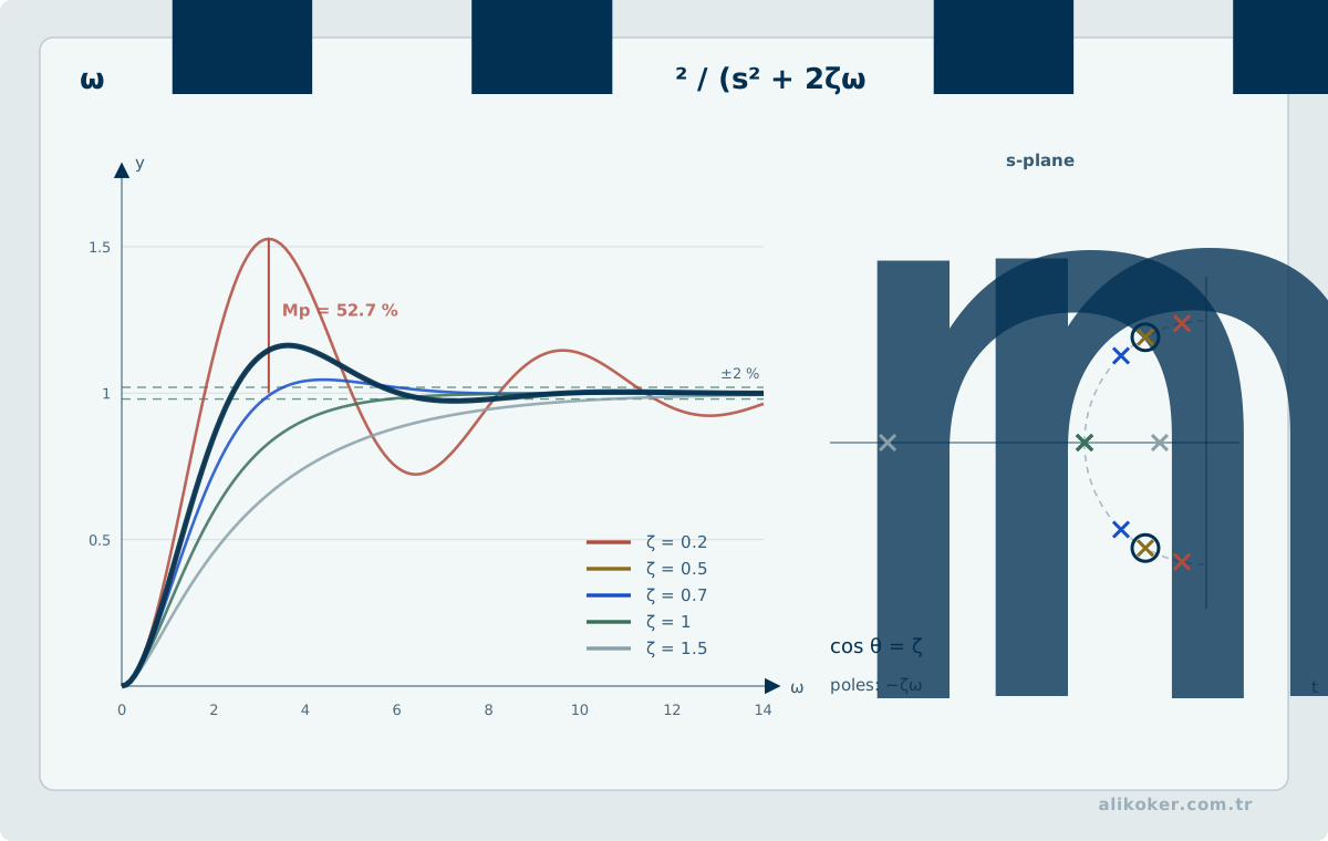
Common measures for a step response include:

Rise time

The time for the output to rise through a specified range toward the target.

t_r

Peak time

The time to reach the first maximum.

t_p

Maximum overshoot

M_p

Settling time

The time after which the output enters and remains within a specified tolerance band.

t_s

Typical bands are:

±2%
or
±5%

30. Approximate second-order relationships

For a standard underdamped second-order system:

ω_d = ω_n sqrt(1-ζ²)

Peak time:

t_p = π / ω_d

Percentage overshoot:

M_p(%) =
100 * exp(
    -ζπ / sqrt(1-ζ²)
)

Approximate 2% settling time:

t_s ≈ 4/(ζω_n)

These relationships are meaningful under assumptions such as:

• dominant second-order behavior,
• standard form,
• limited influence from additional zeros.

31. Dominant poles

In high-order systems, not all poles have equal influence.

Slow poles closer to the imaginary axis often dominate the transient response.

If the fast poles are sufficiently far to the left, the approximation:

high-order system
≈
low-order model

may be used.

Pole-zero proximity and the influence of zeros must nevertheless be checked.

32. Pole-zero cancellation

In theory, a controller zero can cancel a plant pole:

(s+a)/(s+a)

In a real system, however, parameters are never known exactly.

Relying on exact cancellation is particularly risky for unstable or slow poles.

If the model is believed to contain:

s + 1.00

while the real system contains:

s + 0.93

the cancellation is incomplete.

Therefore:

Pole-zero cancellation is an algebraic convenience, not a physical guarantee.

33. Step, ramp, and parabolic inputs

Control systems are commonly examined using standard reference signals.

Step

r(t) = A
R(s) = A/s

This may represent a position reference.

Ramp

r(t) = At
R(s) = A/s²

A reference changing at constant velocity.

Parabola

r(t) = (A/2)t²
R(s) = A/s³

Represents a reference with constant acceleration.

34. Final value theorem

Under appropriate stability conditions:

lim(t→∞) y(t)
=
lim(s→0) sY(s)

may be used.

This theorem is important for calculating steady-state error.

It must not be applied mechanically if right-half-plane poles or inappropriate imaginary-axis behavior are present.

35. Block diagram

Control-system components can be represented with blocks.

Basic elements include:

• block,
• summing junction,
• takeoff point.

Series connection:

G_eq = G1 G2

Parallel connection:

G_eq = G1 + G2

Negative feedback:

        G
T = ----------
     1 + GH

36. Open-loop and closed-loop transfer functions

The loop gain can be written as:

L(s) = G(s)H(s)

The closed-loop transfer function is:

        G(s)
T(s) = -----------
        1 + G(s)H(s)

The characteristic equation is:

1 + G(s)H(s) = 0

The roots of this equation are the closed-loop poles.

37. Stability

Stability is a fundamental requirement in a control system.

Intuitively:

Small initial deviations or bounded inputs should not cause system behavior to grow uncontrollably.

For LTI systems, several notions of stability exist:

• internal stability,
• BIBO stability,
• asymptotic stability.

For a minimal continuous-time rational transfer function, all poles lying in the open left half-plane provides BIBO stability.

38. Marginal stability

Simple poles on the imaginary axis:

s = ±jω

can produce sustained oscillation.

Repeated poles on the imaginary axis can produce growing terms.

Therefore:

Re(p)=0

should not automatically be labeled “stable.”

The type of stability should be stated explicitly.

39. Routh-Hurwitz criterion

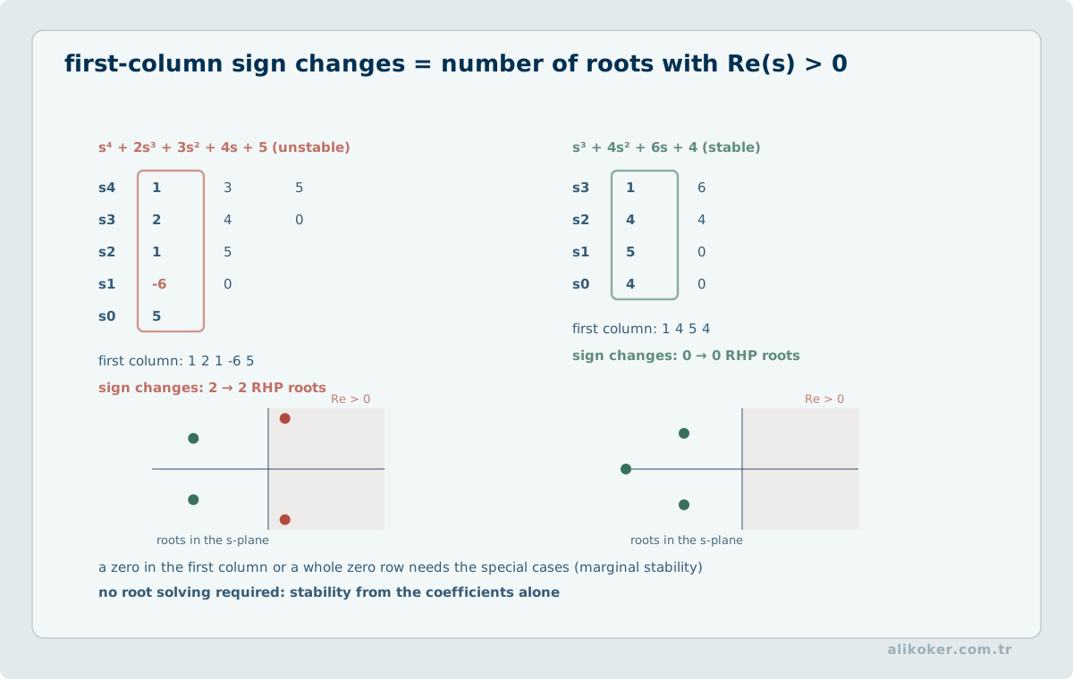
Consider the characteristic polynomial:

a_n s^n + a_(n-1)s^(n-1) + ... + a_0

The Routh array helps determine the number of right-half-plane roots without directly computing the roots.

The central result is:

The number of sign changes in the first column of the Routh array equals the number of right-half-plane roots.

This method is particularly useful for finding the range of a gain parameter that preserves stability.

40. Stability alone is not performance

Two systems can both be stable.

The first may have:

settling = 0.5 s
overshoot = 5%

and the second:

settling = 30 s
overshoot = 70%

Although both are mathematically stable, their engineering quality is not the same.

Control design therefore considers:

stability
+
performance

together.

41. Steady-state error

Let:

e(t) = r(t) - y(t)

The steady-state error is defined as:

e_ss = lim(t→∞) e(t)

This quantity is meaningful when the system is stable and the limit exists.

A common control objective is:

e_ss → 0

42. System type

For a unity-feedback system, the number of integrators at the origin in the open-loop transfer function is called the system type.

If:

L(s) = K / [s^N * ...]

then:

Type = N

The general intuition is:

more integrators
→ higher low-frequency gain
→ lower steady-state error for some references

but also:

phase lag ↑
stability margin ↓

can become a risk.

43. Static error constants

For unity feedback:

Position constant

K_p = lim(s→0) L(s)

Step error:

e_ss = 1/(1+K_p)

Velocity constant

K_v = lim(s→0) sL(s)

For a unit ramp:

e_ss = 1/K_v

Acceleration constant

K_a = lim(s→0) s²L(s)

For a unit parabola:

e_ss = 1/K_a

These relationships assume appropriate closed-loop stability.

44. Fundamental role of integral action

An integral controller:

u_I(t) = K_i ∫ e(t) dt

continues accumulating as long as the error is nonzero.

It is therefore powerful for eliminating steady-state error under a constant reference or constant disturbance.

The integral term, however:

• introduces an additional pole,
• adds phase lag,
• can increase overshoot,
• can produce windup under saturation.

Therefore:

Integral action removes error, but it is not free.

45. Proportional control

A proportional controller is:

u(t) = K_p e(t)

Advantages:

• simple,
• fast,
• stronger action for larger error.

Increasing K_p can often lead to:

response speed ↑
steady-state error ↓

but may also cause:

overshoot ↑
oscillation ↑
risk of instability ↑

The effect of gain should not be memorized independently of the plant.

46. Derivative control

The ideal derivative term is:

u_D(t) = K_d de/dt

The derivative responds:

not only to how large the error is, but also to how fast it is changing.

This can provide damping.

The ideal derivative has:

|G_D(jω)| = K_d ω

and therefore amplifies high-frequency measurement noise.

In real implementations, the derivative is filtered.

47. Filtered derivative

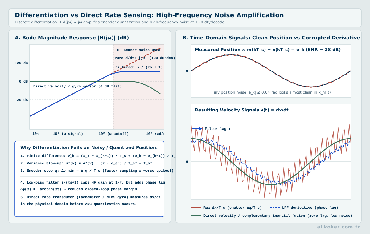
A practical derivative can be written as:

        K_d s
D(s) = --------
       1 + T_f s

or within the PID form:

                  K_d s
C(s)=K_p+K_i/s+------------
                 1+T_f s

Selecting T_f is a tradeoff between:

noise attenuation
↔
preserving derivative action

48. Derivative kick

If the derivative is calculated from error, an abrupt step in the reference:

r(t)

can create a very large short-duration derivative term.

This is called derivative kick.

For this reason, derivative action is often applied to:

the measurement

in practical systems.

For example:

u_D = -K_d dy/dt

This prevents the reference step from being differentiated directly.

49. PI controller

C(s) = K_p + K_i/s

or:

C(s) = K_p(1 + 1/(T_i s))

PI control is widely used in:

• process control,
• motor-speed control,
• current loops.

Because no derivative term is required, it can be simpler than PID with respect to noise.

50. PD controller

C(s) = K_p + K_d s

A PD controller can:

• improve transient response,
• increase damping,
• be useful for fast position control.

Because it contains no integral action, however, it cannot by itself eliminate steady-state error under constant load or disturbance.

51. PID controller

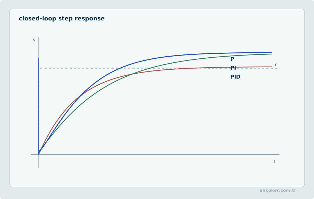
The ideal parallel form is:

u(t) =
K_p e(t)
+
K_i ∫e(t)dt
+
K_d de(t)/dt

The transfer function is:

C(s) = K_p + K_i/s + K_d s

A derivative filter is added in practice.

The effectiveness of PID combines three intuitions:

P → present error
I → accumulated past error
D → error trend

52. What do the PID gains do?

A common starting intuition is:

Kp

speed ↑
error ↓

but overshoot and oscillation may increase.

Ki

Removes steady-state error.

However, it can increase:

• overshoot,
• settling time,
• windup.

Kd

Can increase damping.

However, it:

• is sensitive to measurement noise,
• requires filtering.

These are useful starting intuitions, not universal laws.

53. PID tuning

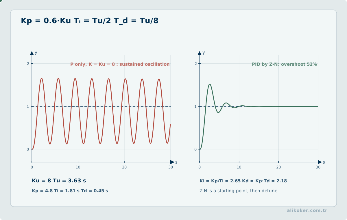
PID tuning appears to be the problem of finding three numbers:

Kp
Ki
Kd

but the design targets must first be defined.

Example requirements:

t_r < 0.5 s
M_p < 10%
t_s < 2 s
e_ss = 0
phase margin > 45°
|u| < 10 V

The gains should satisfy these requirements jointly.

54. Trial-and-error PID tuning

For a simple, low-risk setup:

1. Start with Ki = 0, Kd = 0.
2. Increase Kp.
3. Approach the desired speed of response.
4. Add Kd if more damping is needed.
5. Add Ki if steady-state error remains.
6. Measure the complete response again.

This method can be educational.

Blind trial and error is not suitable, however, for systems that are:

• unstable,
• hazardous,
• high-energy,
• expensive.

55. Ziegler-Nichols

The rules published by Ziegler and Nichols in 1942 are an important milestone in the history of PID tuning.

Two classical approaches are:

• open-loop reaction curve,
• closed-loop ultimate gain.

These methods provide a rapid initial estimate.

In many modern applications, however, they are better regarded as:

an initial tuning

rather than:

the final design.

The resulting response can be aggressive and exhibit high overshoot.

56. Model-based PID tuning

When the model is known, PID gains can be selected through:

• pole placement,
• root locus,
• frequency-domain design,
• optimization,
• robustness objectives.

Current tools can perform automatic PID tuning while targeting a balance among:

stability
performance
robustness

rather than only a “fast response.”

57. Integrator windup

A real actuator has limits.

For example:

-10 V ≤ u ≤ +10 V

Even if the controller calculates:

u_cmd = 40 V

the actuator can apply only:

u_actual = 10 V

Meanwhile, the integral:

∫e dt

may continue accumulating.

When the system approaches the target, the integrator can still contain a very large value and may take a long time to unwind in the opposite direction.

This is called integrator windup.

58. Anti-windup

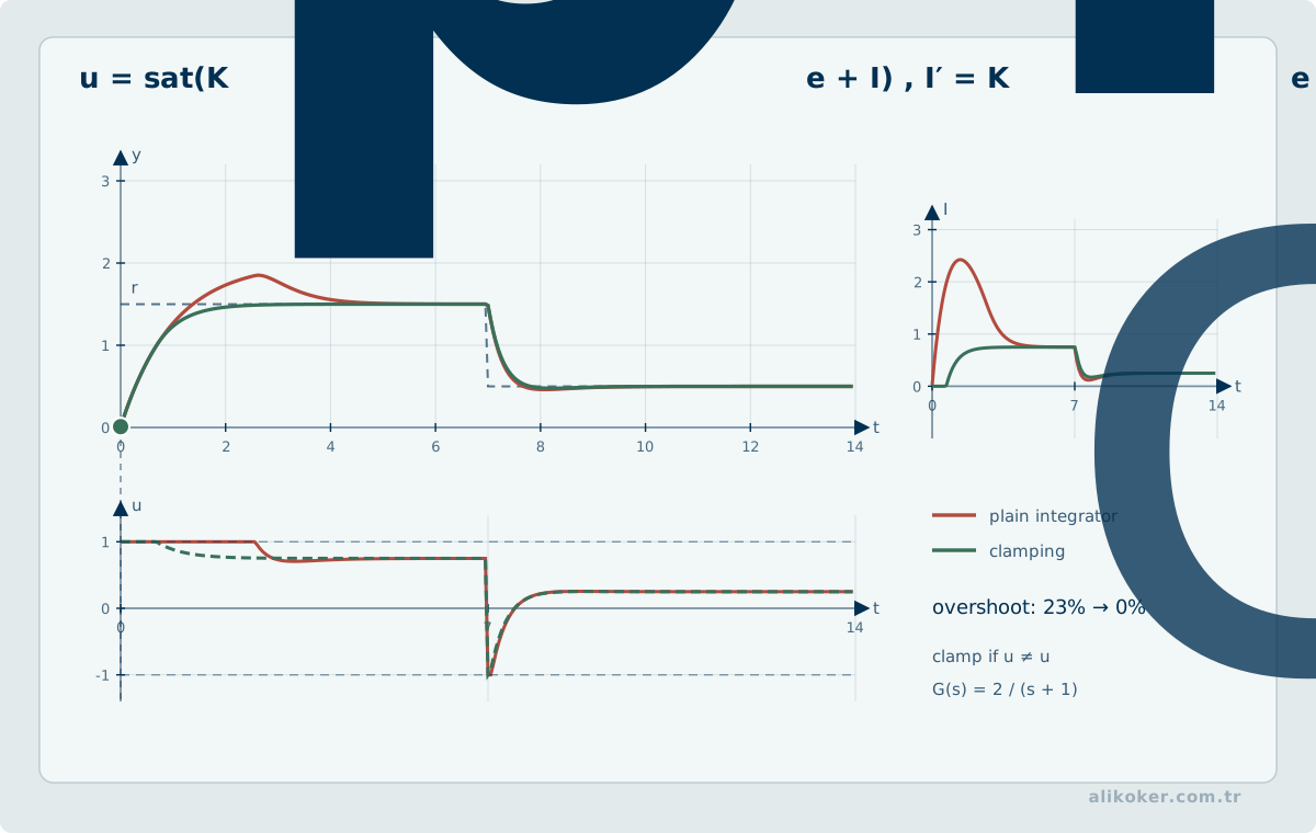
Common anti-windup methods include:

Clamping

When the output is saturated and the error would drive the integrator farther in the wrong direction, integration is stopped.

Back-calculation

The difference between the applied and calculated control is fed back to the integrator:

u_sat - u

This helps unwind the integrator faster.

Tracking

The controller's internal state is arranged to track the control signal actually applied.

Anti-windup is:

not a cosmetic feature added to PID afterward, but part of control design whenever the physical actuator is limited.

59. Saturation

Saturation is not only a PID problem.

Every actuator is limited:

motor torque
valve opening
PWM
current
voltage
heater power
steering angle

A linear model may assume:

u ∈ (-∞,+∞)

while the real system operates under:

u_min ≤ u ≤ u_max

Saturation makes the closed-loop system nonlinear.

60. Rate limiting

Not only actuator magnitude but also its rate of change may be limited:

|du/dt| ≤ r_max

For example:

• large valves,
• steering systems,
• mechanical servos,
• thermal power systems

cannot move instantaneously from one value to another.

Rate limits must be considered in controller design.

61. Two-degree-of-freedom PID

In a one-degree-of-freedom structure, the same PID determines both:

• reference tracking,
• disturbance rejection

through the same error signal.

A two-degree-of-freedom structure can add weighting for the reference.

For example:

u =
K_p(br - y)
+
K_i ∫(r-y)dt
-
K_d dy/dt

Here b can adjust the influence of the reference on the proportional term.

The objective is to tune:

reference response

and:

disturbance rejection

with some degree of independence.

62. Feedforward

Feedback corrects an error after it appears.

Feedforward produces an appropriate action in advance from a known reference or disturbance.

u = u_ff + u_fb

For example, in a robot arm the gravity torque calculated from the model can be compensated in advance using:

u_ff = g(q)

Feedback then corrects the remaining model error.

63. Feedback + feedforward

A good architecture often combines:

model knowledge
+
feedback

Reference → Feedforward ─────┐
                            ↓
                       (+) → Plant
                            ↑
              Feedback ← Output

Feedforward is fast and anticipatory.

Feedback corrects uncertainty.

64. Disturbance rejection

A disturbance:

d(t)

can enter the system at different points.

For example, in a motor system:

load torque

is a disturbance.

A good controller seeks:

d ↑
→ y changes as little as possible

Disturbance rejection should be measured separately from reference tracking.

65. The noise problem

A sensor measures:

y_m = y + n

Because the controller uses this measurement, high loop gain can transfer high-frequency noise into the control signal.

Therefore:

high bandwidth

is not always better.

There is a tradeoff between speed and noise sensitivity.

66. Root locus

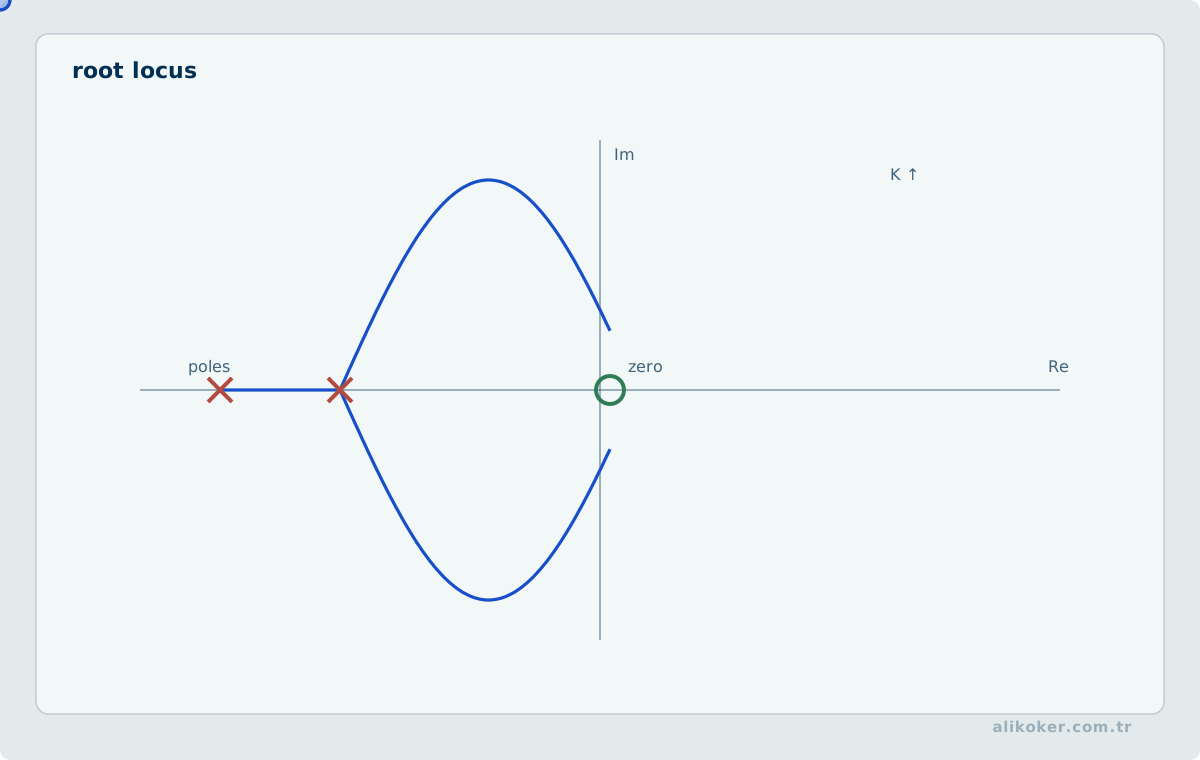
The root locus shows how closed-loop poles move in the complex plane as the open-loop gain changes.

Consider the characteristic equation:

1 + K G(s)H(s) = 0

As K varies over:

0 → ∞

the paths traced by the roots of this equation form the root locus.

67. Purpose of the root locus

The root locus visualizes the question:

How does the closed-loop dynamics change if I change the gain or the controller poles and zeros?

It is therefore a powerful design tool for:

• stability,
• damping,
• speed,
• pole placement.

68. Basic root-locus rules

General rules include:

1. The number of branches equals the number of open-loop poles.
2. Branches start at open-loop poles.
3. They terminate at open-loop zeros or at infinity.
4. Real-axis segments are determined by the angle condition.
5. Asymptotes exist for excess poles.
6. Breakaway and break-in points may be found.
7. Imaginary-axis crossings may be calculated with Routh analysis.

The angle condition is:

∠G(s)H(s) = (2k+1)180°

and the magnitude condition is:

K |G(s)H(s)| = 1

69. Design with root locus

A desired pole location:

s_d = -σ ± jω_d

may be selected from requirements such as:

• damping ratio,
• natural frequency,
• settling time.

Controller poles, zeros, and gain are then added so that the root locus passes through this point.

70. Lead compensator

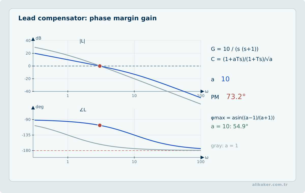
A lead compensator typically has the form:

        s + z
C(s)=K -------
        s + p

with:

|p| > |z|

Aims include:

• increasing phase margin,
• speeding up the response,
• moving poles to the left.

It provides positive phase contribution in the frequency domain.

71. Lag compensator

A lag compensator may be written as:

        s + z
C(s)=K -------
        s + p

and generally uses:

|z| > |p|

to increase low-frequency gain.

The objective is to:

• reduce steady-state error,
• avoid unnecessarily disturbing high-frequency behavior.

The cost can be:

• slower response,
• additional phase lag.

72. Lead-lag

When both transient-response and steady-state-error requirements must be met, lead and lag compensation can be combined:

C(s)=C_lead(s) C_lag(s)

This is one of the important tools of classical control design.

73. Frequency response

If:

u(t) = A sin(ωt)

is applied to an LTI system, the steady-state output at the same frequency is:

y(t) =
A |G(jω)| sin(ωt + ∠G(jω))

Therefore:

|G(jω)| → amplitude ratio
∠G(jω) → phase shift

defines the system's frequency response.

74. Why is the frequency domain important?

Real signals consist of components at different frequencies.

A control system may need to:

at low frequency
track the reference and reject disturbances well

at high frequency
avoid amplifying sensor noise

The frequency domain makes this distinction directly visible.

75. Bode plot

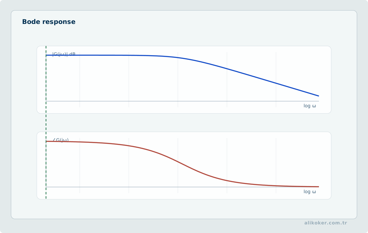
A Bode plot consists of two graphs.

Magnitude

20 log10 |G(jω)|

in dB.

Phase

∠G(jω)

in degrees.

The horizontal axis is logarithmic frequency.

76. Decibel

If the gain is:

M = |G(jω)|

then:

M_dB = 20 log10(M)

For example:

M = 10   → +20 dB
M = 1    → 0 dB
M = 0.1  → -20 dB

The logarithmic representation converts products into sums.

77. Break frequencies

A first-order pole:

1/(1+s/ω_p)

approximately changes the slope as:

ω < ω_p → 0 dB/dec
ω > ω_p → -20 dB/dec

A zero:

1+s/ω_z

contributes:

+20 dB/dec

The Bode plot is therefore a visual language for the pole-zero structure of a system.

78. Resonance

An underdamped second-order system can produce a large amplitude around a particular frequency.

Near this frequency:

|G(jω)|

has a peak.

In flexible mechanical systems, resonance can cause:

• vibration,
• noise,
• fatigue,
• behavior close to instability.

Controller bandwidth should be designed together with the system resonances.

79. Nyquist criterion

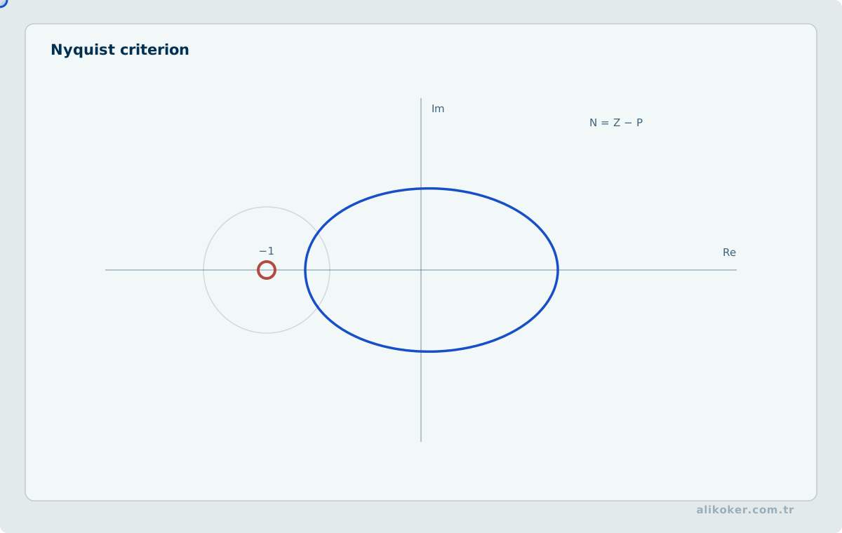
The Nyquist criterion is used to:

determine closed-loop stability from the open-loop frequency response.

Let the loop transfer function be:

L(s)=G(s)H(s)

The characteristic equation is:

1 + L(s)=0

so the critical point is:

L(s) = -1

The number of encirclements of the -1 point by the Nyquist curve, together with the number of open-loop right-half-plane poles, determines closed-loop stability.

80. Sign convention in the Nyquist relation

The sign convention can be written differently in the literature depending on contour orientation.

One common convention is:

N = Z - P

or an equivalent signed form according to the selected direction.

Here:

P → open-loop right-half-plane poles
Z → closed-loop right-half-plane poles
N → net encirclements of -1

It is more important to state the chosen contour and direction convention clearly than to memorize one formula in isolation.

81. Gain margin

Gain margin indicates how far the open-loop gain is from the instability boundary at the frequency where the phase is approximately:

-180°

In general, a larger positive gain margin means:

more tolerance to gain uncertainty

but it is not by itself a guarantee of robustness.

82. Phase margin

At the gain-crossover frequency:

|L(jω_gc)| = 1

if the phase is:

φ

then the phase margin is approximately:

PM = 180° + φ

Phase margin provides practical information about tolerance to:

• delay,
• model error,
• additional dynamics.

83. Bandwidth

Closed-loop bandwidth indicates the frequency range over which the system can adequately follow inputs.

The general intuition is:

bandwidth ↑
→ response speed ↑

but it can also cause:

noise sensitivity ↑
sensitivity to model uncertainty ↑
control effort ↑

Bandwidth is a performance-robustness tradeoff.

84. Delay

A pure time delay:

e^(-Ls)

contributes the phase:

-ωL

without changing magnitude.

The phase becomes increasingly negative as frequency rises.

Therefore delay:

• reduces phase margin,
• limits the maximum practical bandwidth,
• makes fast control more difficult.

Delay can be critical in networked and distributed control systems.

85. Padé approximation

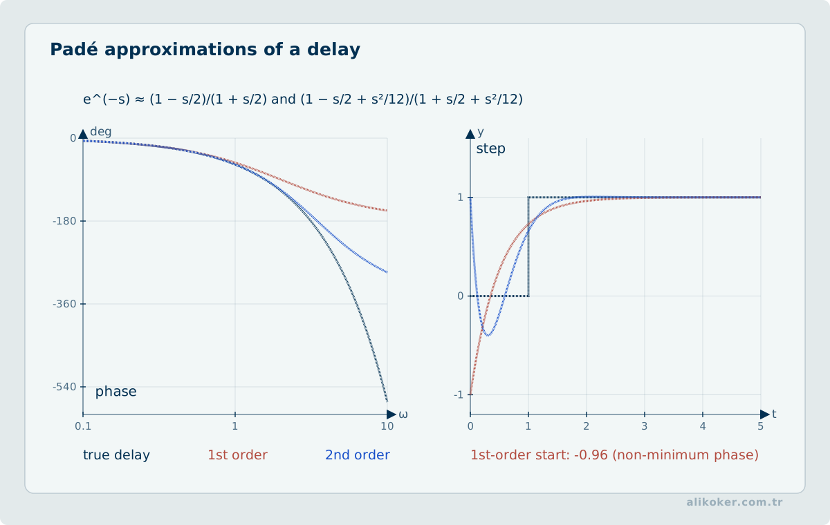
When a delay cannot be represented directly by a classical rational transfer function, a Padé approximation may be used.

The first-order approximation is:

e^(-Ls)
≈
(1 - Ls/2)/(1 + Ls/2)

This is useful for analysis but does not reproduce the exact high-frequency behavior of a true delay.

86. Sensitivity function

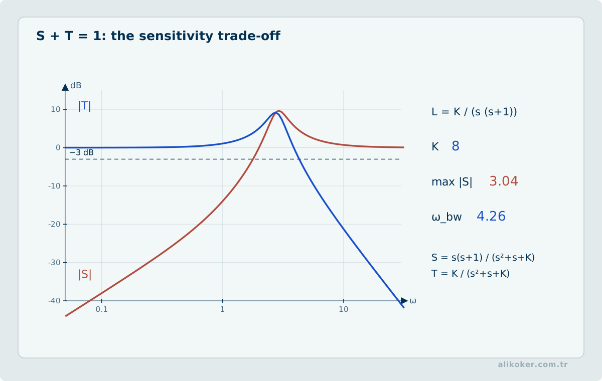
For a unity-feedback structure, let:

L(s) = C(s)P(s)

Sensitivity:

        1
S(s)=-------
       1+L(s)

Complementary sensitivity:

        L(s)
T(s)=-------
       1+L(s)

and:

S(s)+T(s)=1

87. What do S and T represent?

At low frequency, if:

|L| >> 1

then:

S ≈ 0
T ≈ 1

This indicates:

• good reference tracking,
• good rejection of some disturbances.

At high frequency, if:

|L| << 1

then:

S ≈ 1
T ≈ 0

which can reduce the transfer of measurement noise to the closed-loop output.

Good loop shaping often targets:

high gain at low frequency
low gain at high frequency

88. Robustness

The real plant:

P_real(s)

is never exactly identical to the design model:

P_model(s)

Differences may result from:

• parameter tolerances,
• load changes,
• temperature,
• friction,
• aging,
• neglected dynamics.

Robust control aims to preserve closed-loop properties despite these uncertainties.

89. Nominal and robust performance

Nominal performance

Performance when the model is assumed to be exactly correct.

Robust stability

Does the system remain stable in the presence of uncertainty?

Robust performance

Are the performance requirements also maintained under uncertainty?

For a production system, nominal simulation alone is insufficient.

90. Nonminimum-phase system

A right-half-plane zero or certain delays can create nonminimum-phase behavior.

A right-half-plane zero imposes fundamental constraints such as:

• an initial response in the opposite direction,
• bandwidth limitations,
• greater difficulty in aggressive control.

Such dynamics are not defects that can simply be “removed” by a controller; they are physical design constraints.

91. Bode's fundamental limitation idea

Feedback cannot reduce undesirable sensitivity to zero at every frequency simultaneously.

Reducing:

|S| ↓

in one region can have the cost of increasing:

|S| ↑

in another.

This phenomenon is often described as the waterbed effect.

Control design is therefore not about:

maximizing everything at the same time,

but about:

selecting the right priorities across frequency regions.

92. State-space approach

A transfer function represents input-output behavior.

State space represents the internal dynamics as:

ẋ = Ax + Bu
y  = Cx + Du

where:

x → state vector
u → input
 y → output
A → system matrix
B → input matrix
C → output matrix
D → direct-feedthrough matrix

93. What is a state?

A state is the smallest set of variables needed, together with future inputs, to determine a system's future behavior.

For a mass-spring-damper system, for example:

x1 = position
x2 = velocity

can be selected.

Then:

ẋ1 = x2

ẋ2 =
-(k/m)x1
-(b/m)x2
+(1/m)u

or in matrix form:

[ẋ1]   [ 0      1  ][x1]   [  0 ][u]
[ẋ2] = [-k/m -b/m ][x2] + [1/m]

94. Advantages of state space

State space is a natural framework for systems that are:

• multiple-input,
• multiple-output,
• subject to initial conditions,
• time-varying,
• extendable to nonlinear formulations.

Compared with a transfer function, it carries more information about internal dynamics.

95. State-transition matrix

For the homogeneous system:

ẋ = Ax

we have:

x(t) = e^(At)x(0)

With an input:

x(t)
=
e^(At)x(0)
+
∫₀ᵗ e^[A(t-τ)] B u(τ)dτ

e^(At) is the state-transition matrix.

96. Stability in state space

For the continuous-time LTI system:

ẋ = Ax

if all eigenvalues:

λ_i(A)

lie in the left half-plane:

Re(λ_i) < 0

the system is asymptotically stable.

For a minimal state-space realization, these eigenvalues represent the same dynamics as transfer-function poles.

97. Controllability

A system is controllable if its state can be moved to a desired point using a suitable input.

The controllability matrix is:

C =
[B  AB  A²B ... A^(n-1)B]

If:

rank(C) = n

then the system is completely controllable.

98. Why does controllability matter?

If a dynamic mode cannot be influenced by the input:

the controller cannot move that mode to a desired location.

Controllability should therefore be checked before pole placement.

Finding a mathematical controller formula does not by itself mean that the physical system is controllable.

99. Observability

A system is observable if its internal state can be reconstructed from measured inputs and outputs.

The observability matrix is:

O =
[C
 CA
 CA²
 ...
 CA^(n-1)]

If:

rank(O) = n

then the system is completely observable.

100. Why is every state not measured?

In a real system:

position may be measurable
velocity may not be measured directly
current may be measurable
load torque may not be measurable

Measuring every state with sensors can therefore be:

• expensive,
• physically difficult,
• noisy.

The solution is to use a:

state observer

101. State feedback

If the full state is available, a control law such as:

u = -Kx + Nr

may be used.

The closed-loop system becomes:

ẋ = (A-BK)x + BNr

The objective is to place the eigenvalues of:

A-BK

at desired locations.

102. Pole placement

If the system is controllable, an appropriate K can place the closed-loop poles at specified locations.

For example, for desired poles:

-3
-4

one can calculate K such that:

eig(A-BK) = {-3,-4}

Moving the poles as far left as possible is not necessarily good design.

Very fast poles can cause:

• high control effort,
• sensitivity to sensor noise,
• saturation,
• excitation of neglected fast dynamics.

103. State observer

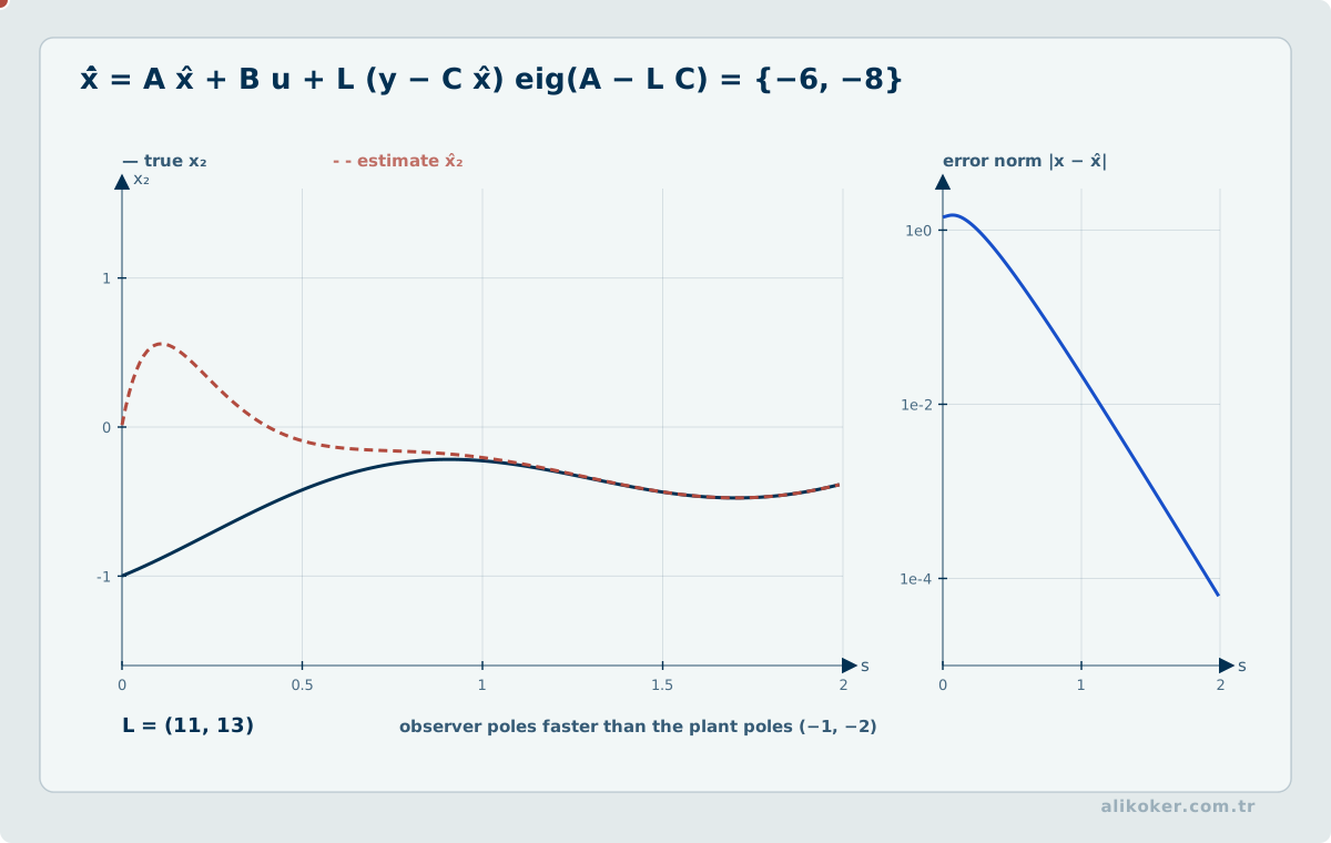
A Luenberger-type observer is:

x̂̇ =
Ax̂ + Bu
+ L(y-Cx̂)

where:

x̂ → estimated state
L  → observer gain

For estimation error:

e_x = x - x̂

we obtain:

ė_x = (A-LC)e_x

L is selected so that the observer-error dynamics are stable and sufficiently fast.

104. Observer poles

Observer poles are often selected faster than controller poles.

An excessively fast observer, however, can:

• amplify measurement noise,
• become sensitive to model error.

There is therefore a tradeoff between:

fast estimation
↔
noise robustness

105. Separation principle

For a linear system, the:

state-feedback gain K

and:

observer gain L

can, under suitable conditions, be designed separately.

The closed-loop eigenvalues:

eig(A-BK)

and observer-error eigenvalues:

eig(A-LC)

together determine system behavior.

This result is known as the separation principle.

106. Kalman filter

The Kalman filter is a fundamental method for state estimation in noisy linear dynamic systems.

Model:

x_(k+1) = A x_k + B u_k + w_k
y_k     = C x_k + v_k

where:

w_k → process noise
v_k → measurement noise

The Kalman filter forms a statistical balance between:

model prediction
+
measurement correction

107. What is a Kalman filter not?

A Kalman filter:

• does not eliminate every kind of noise,
• does not magically correct an incorrect model,
• is not directly sufficient for every nonlinear problem.

Its performance depends on the selected:

model
Q
R

where:

Q → process-noise covariance
R → measurement-noise covariance

108. LQR

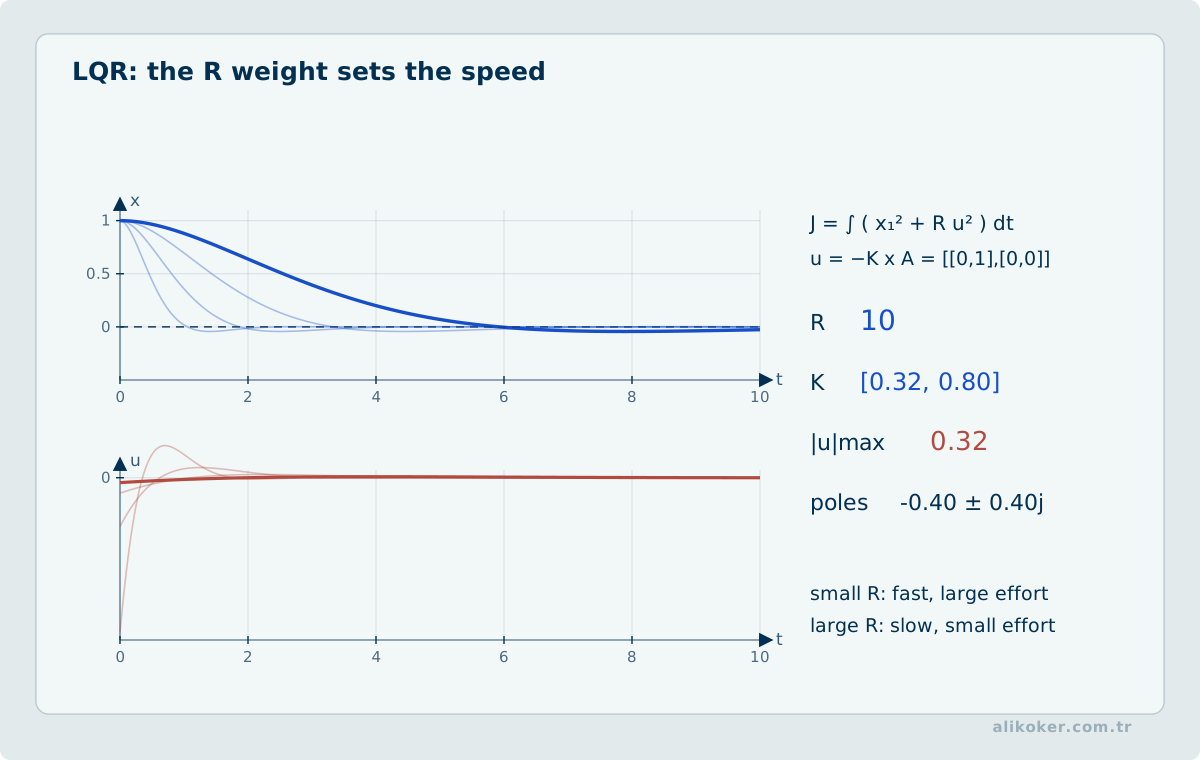
The Linear Quadratic Regulator — LQR determines a state-feedback gain through an optimal-control problem.

The objective is to minimize:

J =
∫₀∞
(xᵀQx + uᵀRu)
dt

where:

Q → penalty on state deviations
R → penalty on control effort

The resulting feedback law is:

u = -Kx

109. Intuition for Q and R

In general:

Q ↑
→ state error is more costly
→ more aggressive control

R ↑
→ control effort is more costly
→ gentler control

The scales of these matrices are affected by physical units.

Choosing Q=I, R=1 is only a starting point.

110. LQG

If all states are not measured, one can combine:

LQR
+
Kalman filter

This structure is known as:

Linear Quadratic Gaussian — LQG

Nominal optimality of LQG does not mean that it:

automatically provides strong robustness margins.

Robustness must be evaluated separately.

111. Multivariable systems

A system with multiple inputs and outputs can be written as:

u ∈ R^m
y ∈ R^p

For a drone, for example:

inputs:
4 motor thrust commands

outputs:
roll
pitch
yaw
altitude

are strongly coupled.

Designing independent SISO loops is not always sufficient.

112. Cross coupling

In a multivariable system:

u1

may influence not only:

y1

but also:

y2, y3...

This is treated as:

• interaction,
• coupling.

Decoupling or MIMO design may be necessary.

113. Nested control loops

Practical systems often use multiple loops.

A servo motor, for example, may have:

innermost loop:
current / torque

middle loop:
speed

outer loop:
position

The general design intuition is:

inner loop faster
outer loop slower

so the outer loop can approximately regard the inner loop as an ideal actuator.

114. Separation of loop bandwidths

An approximate separation may be:

current loop  → 1 kHz
speed loop    → 100 Hz
position loop → 10 Hz

These values are not universal.

The principle is:

the inner loop should be sufficiently faster than the outer loop.

115. Cascade control

The same idea is used in process industries.

For example:

outer:
temperature controller

inner:
steam-flow controller

The inner loop rejects fast disturbances.

The outer loop regulates the primary quality variable.

116. Digital control

Most modern controllers run digitally on:

• microcontrollers,
• PLCs,
• DSPs,
• FPGA-assisted processors,
• industrial computers.

Although the physical system may be continuous-time, the controller samples at:

t = kT_s

117. Sampling

The sampling period is:

T_s

and the sampling frequency is:

f_s = 1/T_s

A digital loop is:

read sensor
↓
compute control
↓
apply output
↓
wait T_s
↓
repeat

118. The Nyquist sampling theorem and control bandwidth are not the same thing

In signal theory:

f_s > 2 f_max

is the fundamental lower bound for avoiding aliasing.

In control applications, merely satisfying this lower bound is generally not enough.

The controller sampling frequency is often selected substantially above the desired closed-loop bandwidth.

A practical initial rule of thumb may be:

f_s ≈ 10...20 × target bandwidth

but:

• delay,
• computational load,
• sensor behavior,
• actuator behavior,
• filtering

must also be examined.

119. Zero-order hold

A digital controller holds its output constant between successive commands.

This behavior is modeled as a zero-order hold — ZOH.

ZOH is a real dynamic element introduced into the continuous plant by digital control.

120. Discrete-time model

A discrete linear system can be written as:

x[k+1] = A_d x[k] + B_d u[k]
y[k]   = C_d x[k] + D_d u[k]

For the continuous model:

ẋ = Ax + Bu

ZOH discretization gives:

A_d = e^(A T_s)

and:

B_d =
∫₀^Ts e^(Aτ)B dτ

121. z-transform

The z-transform plays a role for discrete-time systems analogous to the Laplace transform for continuous-time systems.

A discrete transfer function is:

G(z) = Y(z)/U(z)

While the continuous-time stability region is:

Re(s) < 0

in discrete time it is the interior of the unit circle:

|z| < 1

122. Relationship between the s-plane and z-plane

Sampling is related through:

z = e^(sT_s)

If a continuous-time pole is stable:

Re(s) < 0

then:

|z| < 1

The imaginary axis:

s = jω

maps onto the unit circle.

123. Discrete PID

PID can be implemented directly with difference equations.

For example, the integral may be approximated as:

I[k] =
I[k-1] + K_i T_s e[k]

and the derivative as:

D[k] =
K_d (e[k]-e[k-1])/T_s

A practical implementation should account for:

• filtered derivative action,
• anti-windup,
• output limits,
• sampling jitter.

124. Tustin transformation

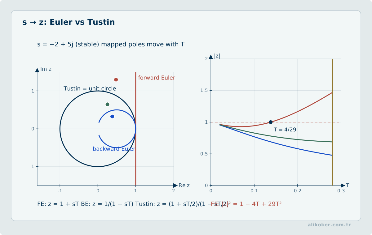
The bilinear transformation can be used to discretize a continuous controller:

s ≈ (2/T_s) (z-1)/(z+1)

This method is known as the Tustin / bilinear transform.

Because it produces frequency warping, prewarping may be used for critical frequencies.

125. Euler methods

Simple discretization methods include:

Forward Euler

s ≈ (z-1)/(T_s z)

with an equivalent finite-difference interpretation.

Backward Euler

This has different stability properties.

Despite their simplicity, the effect of the selected discretization method should be analyzed in high-performance control design.

126. Computational delay

The controller samples the sensor at:

t = kT_s

If the control calculation takes:

T_c

the actuator command is delayed.

This delay creates phase loss.

In a high-bandwidth system:

T_c / T_s

should be kept small.

127. Jitter

If a real-time task is intended to run with:

T_s = 1 ms

but its cycles occur at:

0.8 ms
1.4 ms
0.9 ms
1.2 ms

then the sampling contains jitter.

Jitter can cause:

• phase uncertainty,
• variable delay,
• numerical derivative error.

This is why real-time guarantees matter in control software.

128. Priority inversion and control

In a real-time operating system, a high-priority control task may be delayed by a low-priority task while waiting for a lock.

This is not merely a software-performance issue.

In a high-speed control system:

a scheduling error can become a physical-behavior error.

Control software should therefore be designed with respect to:

• bounded execution time,
• priority policy,
• lock usage,
• watchdogs,
• deadline monitoring.

129. Sensor quantization

ADC measurements have finite resolution.

For example, for a:

12-bit ADC
0-5 V

the resolution is approximately:

5/4096 ≈ 1.22 mV

Small changes in error may remain below this quantization level.

This can cause:

• limit cycles,
• noisy derivative estimates,
• low-speed vibration.

130. Actuator quantization

If PWM is 8-bit over:

0...255

then the control command can take only one of 256 levels.

Small control differences cannot be applied.

This is particularly important in:

• low-speed motion,
• precise positioning,
• mechanisms with friction.

131. Measurement filtering

A low-pass filter can be used for sensor noise.

For example:

          1
F(s)=-----------
      τ_f s + 1

However, filtering produces the tradeoff:

noise ↓
phase lag ↑

Making a filter as aggressive as possible is therefore not good design.

132. Anti-aliasing filter

An analog anti-aliasing filter is required before the ADC to suppress high-frequency components.

A digital filter:

cannot undo aliasing that has already occurred during sampling.

This distinction is especially important in vibration and high-speed sensing systems.

133. Model Predictive Control — MPC

Model Predictive Control predicts future system behavior from a model at every sampling instant and solves an optimization problem.

The general process is:

measure/estimate current state
↓
predict the next N steps
↓
optimize the control sequence
↓
apply only the first control action
↓
obtain a new measurement
↓
optimize again

This is the receding-horizon approach.

134. MPC objective function

A simple example is:

J =
Σ ||y(k+i)-r(k+i)||²_Q
+
Σ ||Δu(k+i)||²_R

The objective balances:

tracking error ↓
control variation ↓

A major strength of MPC is its ability to include physical constraints directly in the optimization problem.

135. MPC constraints

For example, constraints such as:

-10 ≤ u ≤ 10

|Δu| ≤ 1

0 ≤ y ≤ 100

can be defined explicitly.

In PID, saturation is often a nonlinear limit added after the main design; in MPC, constraints can be part of the optimization problem itself.

136. When is MPC strong?

MPC is a strong candidate when the system has:

• multiple variables,
• strong input-output interaction,
• explicit physical constraints,
• slow or medium-speed dynamics,
• known future reference information.

This is an important reason for its historical adoption in chemical and process industries.

137. Cost of MPC

An optimization problem is solved at every sampling instant.

Therefore the following matter:

• computational cost,
• optimization time,
• infeasibility,
• model error,
• solver behavior.

In a real-time system:

solver_time < T_s

must hold not merely on average, but at the required reliability level.

138. Nonlinear MPC

If the model:

ẋ = f(x,u)

is nonlinear, Nonlinear MPC — NMPC may be used.

The optimization then also becomes nonlinear.

Advantages:

• wider operating region,
• better representation of real physical constraints.

Costs:

• higher computational load,
• local minima,
• sensitivity to the initial guess.

139. Adaptive control

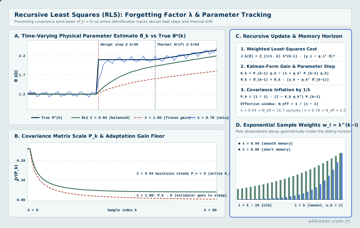
If system parameters change during operation, a fixed controller may become inadequate.

For example, in an aircraft:

speed
altitude
fuel
aerodynamic parameters

and in a motor:

load
temperature
friction

may change.

Adaptive control aims to adjust controller parameters during operation.

140. Gain scheduling

A simpler alternative to a fully adaptive system is:

determine the operating region
↓
select the appropriate controller gains

For example:

low speed  → K1
medium speed → K2
high speed → K3

This structure is called gain scheduling.

Transitions between controllers should consider:

• continuity,
• stability,
• hysteresis.

141. Model Reference Adaptive Control

In MRAC, the desired behavior is defined by a:

reference model

The difference between the actual plant output and reference-model output is used to update controller parameters.

The objective is:

y(t) → y_m(t)

Stability of the adaptation law must be established separately.

142. Nonlinear control

In nonlinear systems:

superposition

does not hold.

A linear controller that performs well near one operating point may fail over a wider region.

Methods include:

• feedback linearization,
• Lyapunov-based control,
• sliding mode,
• backstepping,
• passivity-based control,
• nonlinear MPC.

143. Lyapunov approach

For an equilibrium point, an energy-like function satisfying:

V(x) > 0

is selected.

If:

V̇(x) < 0

then the system can be shown to move toward equilibrium.

The Lyapunov method can provide:

a stability proof without finding the complete solution of the differential equation.

144. Sliding-mode control

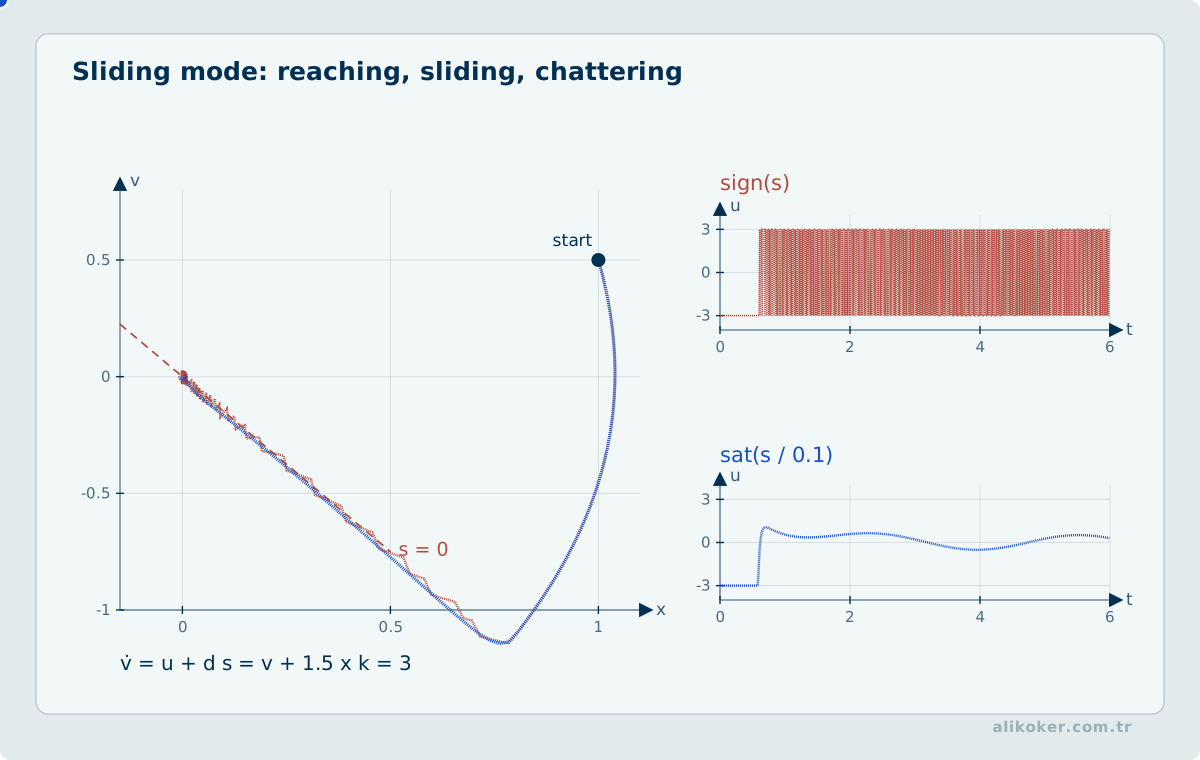
Sliding-mode control defines a sliding surface:

s(x)=0

The state is driven toward this surface and then follows the desired dynamics on it.

Advantage:

• strong robustness to certain matched uncertainties.

Challenges:

• chattering,
• high-frequency switching,
• real actuator limitations.

145. Robust control

Robust control explicitly models uncertainty and seeks stability and performance for:

the entire admissible family of models

Tools include:

• H∞,
• μ-synthesis,
• mixed sensitivity,
• robust loop shaping.

These methods are particularly important in areas such as:

• flight control,
• precision servos,
• flexible structures,
• high-performance mechanical systems.

146. H∞ intuition

The H∞ approach can roughly be viewed as the problem of:

bounding a selected input-output gain under the worst frequency and disturbance direction.

For example, a condition such as:

||T_zw||∞ < γ

may be imposed.

The objective is to limit worst-case gain rather than average behavior.

147. Control effort

How much energy the controller uses can matter as much as whether it reaches the target.

Measures may include:

∫u² dt

or:

Σ u[k]²

An excessively aggressive controller can cause:

• motor heating,
• mechanical wear,
• power loss,
• battery drain.

148. Tracking and disturbance rejection are not the same objective

Reference tracking:

r → y

Disturbance rejection:

d → y

Measurement-noise transfer:

n → y

should be evaluated through different transfer functions.

Declaring the entire system “good” from a single step response is incomplete.

149. Physical constraints in a control system

A real system may have limits such as:

u_min ≤ u ≤ u_max

Δu_min ≤ Δu ≤ Δu_max

y_min ≤ y ≤ y_max

x ∈ safe region

These constraints should be known from the beginning of the design.

In a critical system, an independent safety layer may be required rather than relying on the controller alone.

150. Safety layer

Suppose the normal controller tracks:

T_ref = 90 °C

An independent hardware safety limit can enforce:

T > 120 °C
→ physically disconnect heater power

This separates the functions of:

control

and:

safety

151. Functional safety

IEC 61508 provides a general functional-safety framework for safety functions in electrical, electronic, and programmable electronic systems.

An important distinction for control engineering is:

A normal control function and a safety function are not the same thing.

The normal controller provides performance.

The safety system is designed to bring the plant to a safe state under a specified hazardous condition.

152. Cyber-physical control

A modern control system is not only a physical loop.

It may include:

sensor
network
PLC
controller
SCADA
remote maintenance
historian data
actuator

A cybersecurity vulnerability can therefore become a physical control failure.

153. Cyber threats to control systems

Examples include:

• sensor spoofing,
• changing setpoints,
• modifying actuator commands,
• replay attacks,
• inducing network delay,
• denial of service,
• modifying PLC logic,
• manipulating measurement packets.

Control-system design must consider together:

availability
integrity
safety
timeliness

154. Why is OT security different?

In an information system, actions such as:

stop the service
patch
restart

may sometimes be routine.

In an industrial control system, an abrupt shutdown can cause:

• production loss,
• physical damage,
• safety risk.

NIST SP 800-82 Rev. 3 emphasizes that OT security must be considered together with reliability, performance, and safety requirements.

155. Time in control communication

Correct packet contents are not sufficient.

Control requires:

correct value
+
value at the correct time

For a fast system, correct sensor information arriving 100 ms late can be as harmful as an incorrect decision.

Therefore:

• latency,
• jitter,
• packet loss,
• clock synchronization

are part of control-system reliability.

156. Fault tolerance

A sensor fault may appear as:

stuck value
bias
drift
disconnection
outlier

An actuator fault may include:

stuck
loss of effectiveness
saturation

Fault-tolerant control:

• detects the fault,
• isolates it,
• reconfigures the system when possible.

157. Sensor validation

A single sensor value should not be trusted blindly.

Methods include:

• physical-range checks,
• rate-of-change limits,
• comparison of two sensors,
• model-based residuals,
• majority voting.

For example, if:

|y_measured - y_predicted| > threshold

then a fault candidate may be flagged.

158. Watchdog

If a real-time controller fails to complete its cycle within the specified time, a watchdog may:

• reset the system,
• enter a safe mode,
• switch to a backup controller.

A watchdog:

does not replace a stability proof; it is an additional safety layer against software or hardware failures.

159. Fail-safe and fail-operational

Fail-safe

On failure, the system moves to a safe state.

For example:

heater → off

Fail-operational

A specified function continues even after a failure.

A critical flight-control system, for example, may switch to a redundant channel.

The choice depends on:

• risk analysis,
• physical process,
• mission requirements.

160. Practical sequence for controller design

A sound automatic-control project can follow:

1. Define the control objective
2. Identify inputs and outputs
3. State physical limits
4. Select sensors and actuators
5. Build a model
6. Validate the model experimentally
7. Define the operating point
8. Quantify performance requirements
9. Select an appropriate control architecture
10. Design the controller
11. Add saturation and noise effects
12. Simulate
13. Perform robustness analysis
14. Validate the real-time implementation
15. Test safety and fault scenarios
16. Commission the hardware gradually

This sequence turns control from merely solving equations into a systems-engineering problem.

161. Why is simulation not enough?

Simulation is:

• fast,
• repeatable,
• safe for testing hazardous scenarios.

But simulation remains inside the model.

The real system contains details such as:

sensor noise
cable resistance
friction
backlash
saturation
dead zone
power-supply limits
timing delay
quantization
mechanical flexibility

Therefore:

A controller that works in simulation is evidence that it can work on the real system, not proof that it will.

162. Model-in-the-Loop

At the first stage:

controller model
+
plant model

run in the same simulation environment.

This can be called:

Model-in-the-Loop — MIL

The objective is to evaluate rapidly:

• the control architecture,
• initial gains,
• performance targets.

163. Software-in-the-Loop

The actual controller code or production-near software is run against:

the simulated plant

The objective is to validate:

• differences between algorithm and implementation,
• numerical precision,
• software logic.

164. Processor-in-the-Loop

The controller code runs on the target processor while the physical process remains simulated.

This stage is valuable for evaluating:

• execution time,
• floating- versus fixed-point effects,
• target compiler behavior,
• numerical behavior.

165. Hardware-in-the-Loop

Real control hardware is connected to a:

real-time process simulator

HIL allows conditions such as:

• faults,
• excessive inputs,
• sensor disconnection,
• communication delay,
• boundary conditions

to be tested without damaging the physical process.

166. Commissioning

Transition to the real system should be gradual.

An example sequence is:

1. Monitor sensors only
2. Verify scaling
3. Test the actuator open-loop at low power
4. Verify sign conventions
5. Enable safety limits
6. Enter closed-loop operation with low gain
7. Use a small reference
8. Perform a disturbance test
9. Gradually expand the operating range
10. Perform final performance tests

Sign errors are particularly dangerous.

A loop intended to provide negative feedback can become positive feedback because of incorrect wiring or a software sign error.

167. DC motor speed control

A DC motor is a powerful experimental platform for teaching automatic control.

Input:

motor voltage / PWM

Output:

ω

Disturbance:

load torque

An initial objective may be:

ω → ω_ref

168. DC motor speed experiment

A practical exercise:

1. Drive the motor open-loop.
2. Measure the PWM-speed relationship.
3. Apply step inputs.
4. Obtain an approximate first-order model.
5. Design a PI controller.
6. Test a reference step.
7. Add mechanical load.
8. Measure disturbance rejection.

Measures can include:

rise time
settling time
overshoot
e_ss
peak current

169. DC motor position control

Because motor position satisfies:

θ̇ = ω

an integrator is added to the speed dynamics.

For position control, the following approaches can be compared:

• P,
• PD,
• PID,
• state feedback.

The role of integral action becomes particularly clear under constant load torque.

170. Observing derivative action on a motor

If position control uses only a high Kp, it can produce:

• fast motion,
• overshoot,
• oscillation.

Adding velocity feedback or derivative action:

-K_d θ̇

can create behavior similar to mechanical damping.

This experiment provides a strong intuitive demonstration of P and D action.

171. Flexible mechanism

Flexibility between two masses or two shafts creates resonance.

A simple servo model may appear sufficient while the real system:

motor
↓
flexible coupling
↓
load

can produce high-frequency oscillation.

This experiment demonstrates:

• resonance,
• flexible modes,
• bandwidth limits,
• risks of model reduction.

172. Poor design in a flexible system

If an aggressive PID is designed using only a low-frequency motor model, the controller can excite:

the neglected resonant mode

The result may be:

• vibration,
• noise,
• instability,
• mechanical damage.

The frequency range used for system identification should therefore extend beyond the intended control bandwidth.

173. Magnetic levitation

A magnetic-levitation system is a classical nonlinear and open-loop unstable system.

Electromagnetic force may approximately follow a nonlinear relation such as:

F_m ∝ i²/x²

and is balanced against gravity:

mg

The system can be linearized around an equilibrium point and a controller designed for that region.

174. Why magnetic levitation is instructive

This setup combines:

• open-loop instability,
• operating point,
• linearization,
• fast sensing,
• inner current loop,
• outer position loop.

The fact that the object cannot remain balanced when the controller is disabled directly demonstrates the physical importance of feedback.

175. Ball-and-beam system

The position of a ball on a beam is controlled through:

beam angle

There are nested dynamics between ball position and the servo.

The system is useful for teaching:

• multi-loop control,
• unstable or weakly damped behavior,
• position measurement,
• nonlinear modeling.

176. Inverted pendulum

An inverted pendulum has an open-loop unstable equilibrium.

The objective is:

θ → 0

and, in many setups, simultaneously:

x → x_ref

This is a classical laboratory system for:

• state space,
• controllability,
• LQR,
• observers,
• nonlinear swing-up.

177. Furuta pendulum

A Furuta pendulum consists of a rotary arm and pendulum.

Input:

arm motor torque

Possible states are:

arm angle
arm angular velocity
pendulum angle
pendulum angular velocity

Although the system has a single input rather than being MIMO, its internal dynamics are strongly coupled.

178. Swing-up and stabilization

An inverted pendulum contains two different control problems.

Swing-up

Inject energy to move the pendulum from the downward position to the upright region.

Stabilization

Suppress small deviations around the upright equilibrium.

A single linear controller generally cannot solve both tasks over the full range.

A hybrid structure may use:

energy-based swing-up
↓
enter the balance region
↓
LQR / state feedback

179. Temperature control

Thermal systems are generally slower than mechanical systems.

A simple model:

C_th dT/dt
=
P_heater
-
(T-T_amb)/R_th

can approximate first-order behavior.

Such a system provides a safe, slow experiment for teaching PI/PID control.

180. Important realities of thermal systems

• a heater may provide only positive power,
• cooling may be passive,
• delay may be large,
• sensor location matters,
• thermal inertia may be high.

The symmetric assumption u ∈ (-∞,+∞) is therefore often incorrect.

181. Level control

A tank can be modeled as:

A dh/dt = q_in - q_out

If the outflow satisfies:

q_out ∝ sqrt(h)

then the system is nonlinear.

It can be linearized around an operating point.

Level control is suitable for teaching:

• process dynamics,
• integral behavior,
• valve saturation,
• cascade control.

182. Basic loop for control software

A minimal embedded-controller structure is:

every Ts:
    measurement = read_sensor();

    filtered = filter(measurement);

    error = reference - filtered;

    control = controller(error);

    control = apply_limits(control);

    write_actuator(control);

    monitor_faults();

The parts that are as important as the mathematical controller itself are:

filter
limits
timing
fault monitoring

183. PID pseudocode

error = reference - measurement

P = Kp * error

integral += Ki * Ts * error

derivative =
    filtered_derivative(measurement)

u_raw =
    P
    + integral
    - Kd * derivative

u =
    clamp(u_raw, u_min, u_max)

anti_windup(u, u_raw)

This structure illustrates the transition from ideal textbook PID to production PID.

184. Data logging in the control loop

At minimum, the following should be logged:

timestamp
reference
measurement
error
control_raw
control_applied
integral_state
saturation_flag
fault_flags

An advanced system may also log:

• estimated state,
• raw sensor data,
• delay,
• cycle execution time.

Without data logging, tuning a real system becomes largely guesswork.

185. Plots for control performance

A single output plot is insufficient.

An experiment should show at least:

Reference and output

r(t), y(t)

Error

e(t)

Control signal

u(t)

Saturation

u_raw vs u_applied

A controller that tracks the target well while remaining continuously saturated may not be well designed.

186. Step test

A step response rapidly reveals:

• speed,
• damping,
• steady-state error,
• saturation,
• nonlinearity.

By itself, however, it provides insufficient information about:

• noise robustness,
• frequency limits,
• different operating points.

187. Disturbance test

Keep the reference constant and apply a known disturbance.

For a motor:

add mechanical load

For a heater:

open the door / create airflow

Measure:

maximum deviation
recovery time
steady-state error

This test demonstrates actual regulation performance.

188. Noise test

As control bandwidth increases, the influence of sensor noise on:

u(t)

should be observed.

Especially with derivative action, one may evaluate:

control RMS

and the power spectrum.

189. Parameter-variation test

Simulation can vary model parameters by:

±10%
±20%

On the real system one can vary:

• load,
• supply voltage,
• temperature.

The purpose is to determine how robust the nominal design is.

190. Worst-case approach

Only evaluating:

average performance

may be insufficient.

In a critical system, combinations such as:

maximum delay
minimum voltage
maximum load
sensor tolerance
worst friction

should be considered together.

The controller must remain safe under the worst valid operating condition.

191. Basic linear model in MATLAB

Example:

s = tf('s');

P = 1/(s^2 + 2*s + 5);

step(P);
grid on;

Poles and zeros:

pole(P)
zero(P)

Frequency response:

bode(P);
margin(P);

Root locus:

rlocus(P);

192. PID in MATLAB

C = pid(Kp,Ki,Kd);

T = feedback(C*P,1);

step(T);

Automatic initial tuning:

C = pidtune(P,'PID');

The current Control System Toolbox also supports methods such as:

• PID/PIDF,
• 2-DOF PID,
• Bode loop shaping,
• root locus,
• LQR/LQG,
• Kalman design.

An automatically tuned result should not be deployed before physical limits are incorporated.

193. State space in MATLAB

A = [0 1; -5 -2];
B = [0; 1];
C = [1 0];
D = 0;

sys = ss(A,B,C,D);

Controllability:

rank(ctrb(A,B))

Observability:

rank(obsv(A,C))

Pole placement:

K = place(A,B,[-3 -4]);

194. LQR in MATLAB

Q = diag([10 1]);
R = 0.5;

K = lqr(A,B,Q,R);

Then:

Acl = A - B*K;

and the closed-loop eigenvalues can be examined.

At this point, not only eig(Acl) but also:

• control effort,
• saturation,
• step response,
• model variation

should be tested.

195. Control analysis with Python

The Python ecosystem supports basic analysis with python-control, SciPy, and NumPy.

Example:

import control as ct

P = ct.tf([1], [1, 2, 5])

ct.poles(P)
ct.zeros(P)
ct.step_response(P)
ct.bode_plot(P)

Closed loop:

C = ct.pid(1, 1, 0.1)  # The method may differ by API version
T = ct.feedback(C * P, 1)

The current API of the library version in use should be verified.

196. Tools do not eliminate theory

Software can calculate the results of:

pidtune
place
lqr
margin
rlocus

But it does not automatically decide:

• which model is correct,
• which operating point matters,
• which bandwidth is safe,
• whether sensor noise is acceptable,
• what actuator limits apply,
• which performance metric matters,
• whether failure is safe.

Control engineering is the complete set of these decisions.

197. Artificial intelligence and control engineering

Artificial intelligence can:

• help derive model equations,
• generate code,
• analyze logs,
• suggest parameter sweeps,
• summarize experimental results,
• compare control literature.

In a critical control loop, however:

“the model suggested it”

is not a proof of stability or safety.

The control law must be validated mathematically and experimentally.

198. Learning-based control

Machine learning can be incorporated into control systems for:

• system identification,
• estimation of unknown dynamics,
• gain scheduling,
• estimation,
• policy learning.

But learning-based control increases challenges such as:

• out-of-distribution operation,
• stability guarantees,
• safe exploration,
• explainability,
• computation time.

199. Reinforcement Learning and control

In reinforcement learning, a policy:

u = π(x)

can be learned to maximize a reward.

This approach can be powerful in some high-dimensional tasks.

The distinction from classical control matters.

Classical design generally proceeds from:

model
+ stability
+ performance requirement

whereas RL learns a policy from:

experience
+ reward
+ optimization

Safe training is a separate problem for critical physical systems.

200. Safe use of learning-based control

A safer hybrid architecture may be:

verified safe baseline controller
+
learning-based improvement layer
+
hard safety limits

For example, the learning layer may perform:

• feedforward adaptation,
• model-error compensation,
• parameter estimation,

while fundamental stabilization remains in a verified controller.

201. Digital twin

In a control context, a digital twin can be viewed as:

physical system
+
computational model updated with current data

Possible uses include:

• state monitoring,
• prediction,
• controller testing,
• fault scenarios,
• maintenance planning.

Its control value depends on how current and well validated the model remains against the real system.

202. Simplicity in automatic control

Unnecessary complexity often adds no value in control design.

If a simple PI:

meets the requirements

then using MPC is not technical superiority.

A sound sequence is:

simplest sufficient model
↓
simplest sufficient controller
↓
measure
↓
increase complexity only when necessary

203. When is a simple controller better?

PI/PID is often the best engineering solution when there is:

• a well-understood process,
• few inputs and outputs,
• weak constraints,
• low interaction,
• generous robustness margin,
• easy maintenance.

In production:

a simple, understandable, verified system

is often more valuable than:

a theoretically more advanced but fragile system.

204. When is a complex method justified?

MPC, robust control, or nonlinear methods may be justified when:

• classical PID cannot meet the objectives,
• multivariable interactions are strong,
• constraints dominate the problem,
• the operating range is wide,
• model uncertainty is large,
• safety constraints need to be incorporated in optimization.

The method should be only as complex as the problem requires.

205. Thinking of the control system in layers

A practical architecture may be:

Mission / planning
↓
Reference generation
↓
Outer control loop
↓
Inner control loop
↓
Actuator control
↓
Power electronics
↓
Physical system
↓
Sensor
↓
State estimation

Alongside it may run:

safety monitor
fault detection
telemetry
watchdog

This structure more closely reflects real modern mechatronic systems.

206. Main questions for a control engineer

When examining a system, ask in order:

What is being controlled?
What is being measured?
What can be actuated?
What is the reference?
What are the disturbances?
What is the model?
What is the operating region?
How will stability be demonstrated?
How will performance be measured?
What are the physical limits?
How large are noise and delay?
What happens if the model is wrong?
What happens if a sensor fails?
What happens if the controller misses its deadline?

If these questions have no answers, discussing PID gains is premature.

207. Exercise 1 — first-order system

Given:

        2
G(s)=-------
       3s+1

1. find the time constant,
2. find the DC gain,
3. write the unit-step response,
4. estimate the 2% settling time,
5. compare the unity-feedback system for Kp=1, 5, 20.

208. Exercise 2 — second-order system

For:

             25
G(s)=----------------
       s²+4s+25

calculate:

1. ω_n,
2. ζ,
3. ω_d,
4. overshoot,
5. peak time,
6. settling time.

Compare the approximate relationships with simulation.

209. Exercise 3 — Routh

Let the characteristic equation be:

s³ + 4s² + 3s + K = 0

Construct the Routh array.

Find the stable range of K.

Verify the same range by numerically computing the poles.

210. Exercise 4 — root locus

For:

          K
L(s)=--------------
       s(s+2)(s+5)

1. show the poles,
2. identify the real-axis segments,
3. find the asymptotes,
4. find the imaginary-axis crossing using Routh analysis,
5. select an operating point near the ζ=0.7 line.

211. Exercise 5 — PI

Use the DC motor speed model:

        K
P(s)=-------
       τs+1

Design a PI controller:

C(s)=Kp+Ki/s

Test separately:

reference step
load-torque disturbance
measurement noise

Do not rely on a single plot.

212. Exercise 6 — anti-windup

Consider the first-order system:

P(s)=1/(10s+1)

with saturation:

-1 ≤ u ≤ 1

Run the same PID:

1. without anti-windup,
2. with clamping,
3. with back-calculation.

Compare:

integral state
overshoot
recovery time

213. Exercise 7 — frequency domain

For the open-loop system:

L(s)=10/[s(s+1)(0.1s+1)]

plot the Bode diagram.

Find:

• gain crossover,
• phase crossover,
• phase margin,
• gain margin.

Explain how the margins change when the gain is doubled.

214. Exercise 8 — delay

Add the delay:

e^(-Ls)

to the same system.

Compare phase margin for:

L = 0
0.05
0.1
0.2 s

Explain why delay can degrade stability without changing magnitude.

215. Exercise 9 — state feedback

For:

A = [[0,1],[-2,-3]]
B = [[0],[1]]

1. test controllability,
2. place the poles at {-4,-5},
3. find K,
4. measure the peak control signal,
5. move the poles to {-20,-25} and demonstrate why faster is not always better.

216. Exercise 10 — observer

For the same system, let:

C = [1,0]

1. test observability,
2. select observer poles {-8,-9},
3. introduce an initial estimation error,
4. add sensor noise,
5. move the observer poles far to the left and inspect the noise effect.

217. Exercise 11 — LQR

For a mass-spring-damper system, try the combinations:

Q1 = diag(1,1)
Q2 = diag(100,1)
R1 = 1
R2 = 10

For each design, measure:

• settling time,
• position error,
• maximum control effort,
• ∫u²dt.

Demonstrate that the word “optimal” depends on the chosen cost function.

218. Exercise 12 — sampling

Discretize the continuous controller with:

Ts = 1 ms
10 ms
50 ms
100 ms

On the same physical process, examine changes in:

• stability,
• overshoot,
• phase margin,
• control signal.

219. Exercise 13 — MPC

Construct a two-input, two-output system.

Let the constraints be:

-2 ≤ u1,u2 ≤ 2
|Δu| ≤ 0.2

Using MPC, compare:

1. the unconstrained solution,
2. the constrained solution,
3. a shorter prediction horizon,
4. a longer prediction horizon.

220. Exercise 14 — safety

For a temperature-control system, define:

normal target = 80 °C
warning = 100 °C
critical limit = 120 °C

Handle the following cases separately:

• PID control,
• sensor stuck-at fault,
• actuator stuck-on fault,
• controller-software lockup.

Design the distinction between normal control and an independent safety interlock.

221. Exercise 15 — cyber-physical attack

Add a bias attack to sensor data in the closed-loop model:

y_attack = y + b

Then simulate:

replay
delay
packet loss

Measure:

• error,
• control signal,
• safe-limit violations,
• residual-based detection time.

222. Quick reference

When designing an automatic-control system, ask:

1. What is the plant?
2. What is the output?
3. What is the manipulated input?
4. What is the reference?
5. What are the disturbances?
6. What does the sensor measure and with what accuracy?
7. What are the actuator limits?
8. Over which operating region is the model valid?
9. Is the open-loop system stable?
10. How will closed-loop stability be verified?
11. Are transient-response objectives quantitative?
12. What is the steady-state error requirement?
13. What should the bandwidth be?
14. Are gain and phase margins sufficient?
15. How much noise is present?
16. How much delay and jitter are present?
17. Have saturation and anti-windup been addressed?
18. Has model uncertainty been tested?
19. Is safe behavior under faults defined?
20. Has the real system been tested in addition to simulation?

223. Conclusion

The fundamental idea of automatic control is simple:

Know the desired behavior.
Measure the actual behavior.
Reduce the difference.
Measure again.

Turning this simple loop into a reliable engineering system requires a combination of:

physics
+
mathematics
+
signal processing
+
electronics
+
software
+
real-time engineering
+
safety

The classical chain of control theory:

differential equation
→ transfer function
→ poles and zeros
→ stability
→ time response
→ root locus
→ frequency response

has expanded in modern control to include:

state space
→ observer
→ optimal control
→ robust control
→ MPC
→ nonlinear / adaptive control

The central problem remains unchanged:

Driving a real system with uncertainty and disturbances toward desired behavior, stably and measurably, while respecting physical constraints.

One of the most dangerous misconceptions in control engineering is:

simulation looks good
→ system is ready

The real engineering sequence is:

Model
↓
Design
↓
Analyze
↓
Simulate
↓
Add constraints
↓
Add disturbances
↓
Add uncertainty
↓
Validate real-time behavior
↓
Test gradually on hardware
↓
Measure
↓
Redesign if necessary

Final principle:

A good controller is not the most complex controller. It is the simplest controller that verifiably satisfies the requirements.

References

Sources published after the original publication date were used in the September 2026 revision for technical verification and current tool or standards information.

Primary source

1. Hernández-Guzmán, V. M.; Silva-Ortigoza, R. Automatic Control with Experiments. Advanced Textbooks in Control and Signal Processing, Springer, 2019.

DOI series: https://doi.org/10.1007/978-3-319-75804-6 This source was used in the September 2026 revision as a reference for feedback, physical modeling, transfer functions, Routh analysis, root locus, frequency response, state space, and experimental platforms.

Classical works

1. Maxwell, J. C. “On Governors.” Proceedings of the Royal Society of London, 1868.

1. Routh, E. J. A Treatise on the Stability of a Given State of Motion. 1877.

1. Hurwitz, A. “Über die Bedingungen, unter welchen eine Gleichung nur Wurzeln mit negativen reellen Teilen besitzt.” Mathematische Annalen, 1895.

1. Minorsky, N. “Directional Stability of Automatically Steered Bodies.” Journal of the American Society for Naval Engineers, 1922.

1. Black, H. S. Negative-feedback amplifier work and patents, Bell Telephone Laboratories, 1920s-1930s.

1. Nyquist, H. “Regeneration Theory.” Bell System Technical Journal, 1932.

1. Ziegler, J. G.; Nichols, N. B. “Optimum Settings for Automatic Controllers.” Transactions of the ASME, 1942.

1. Bode, H. W. Network Analysis and Feedback Amplifier Design. Van Nostrand, 1945.

1. Evans, W. R. “Graphical Analysis of Control Systems.” Transactions of the AIEE, 1948.

1. Kalman, R. E. “A New Approach to Linear Filtering and Prediction Problems.” Journal of Basic Engineering, 1960.

Core textbooks

1. Ogata, K. Modern Control Engineering. Prentice Hall.

1. Dorf, R. C.; Bishop, R. H. Modern Control Systems. Pearson.

1. Franklin, G. F.; Powell, J. D.; Emami-Naeini, A. Feedback Control of Dynamic Systems. Pearson.

1. Åström, K. J.; Murray, R. M. Feedback Systems: An Introduction for Scientists and Engineers. Princeton University Press / Caltech open edition.

https://fbsbook.org/

1. Åström, K. J.; Hägglund, T. Advanced PID Control. ISA.

1. Skogestad, S.; Postlethwaite, I. Multivariable Feedback Control: Analysis and Design. Wiley.

Modern and advanced control

1. Khalil, H. K. Nonlinear Systems. Prentice Hall.

1. Slotine, J.-J. E.; Li, W. Applied Nonlinear Control. Prentice Hall.

1. Zhou, K.; Doyle, J. C.; Glover, K. Robust and Optimal Control. Prentice Hall.

1. Rawlings, J. B.; Mayne, D. Q.; Diehl, M. Model Predictive Control: Theory, Computation, and Design. Nob Hill Publishing.

1. Ioannou, P. A.; Sun, J. Robust Adaptive Control. Dover.

Current technical documentation and tools

1. MathWorks. Control System Toolbox Documentation.

https://www.mathworks.com/help/control/

1. MathWorks. PID Controller Tuning.

https://www.mathworks.com/help/control/pid-controller-design.html

1. MathWorks. Anti-Windup Control Using PID Controller Block.

https://www.mathworks.com/help/simulink/slref/anti-windup-control-using-a-pid-controller.html

1. MathWorks. Model Predictive Control Toolbox Documentation.

https://www.mathworks.com/help/mpc/

1. Python Control Systems Library.

https://python-control.readthedocs.io/

Safety and critical systems

1. NIST. SP 800-82 Rev. 3 — Guide to Operational Technology (OT) Security. September 2023.

https://csrc.nist.gov/pubs/sp/800/82/r3/final

1. IEC. IEC 61508:2010 — Functional Safety of Electrical/Electronic/Programmable Electronic Safety-Related Systems.

1. IEC. IEC 62443 Series — Security for Industrial Automation and Control Systems.

Quick formula reference

Error:
e(t)=r(t)-y(t)

Negative feedback:
T(s)=G(s)/(1+G(s)H(s))

First order:
G(s)=K/(τs+1)

Second order:
G(s)=ωn²/(s²+2ζωn s+ωn²)

Damped frequency:
ωd=ωn√(1-ζ²)

Peak time:
tp=π/ωd

2% settling time:
ts≈4/(ζωn)

Overshoot:
Mp=exp[-ζπ/√(1-ζ²)]

PID:
C(s)=Kp+Ki/s+Kd s

Sensitivity:
S=1/(1+L)

Complementary sensitivity:
T=L/(1+L)

State space:
ẋ=Ax+Bu
y=Cx+Du

State feedback:
u=-Kx

Observer:
x̂̇=Ax̂+Bu+L(y-Cx̂)

Discrete system:
x[k+1]=Ad x[k]+Bd u[k]

Continuous-discrete pole relation:
z=e^(sTs)

References

- Albert-László Barabási. Network Science.
- Petter Holme; Jari Saramäki (eds.). Temporal Network Theory. 2nd ed. Springer Nature Switzerland, 2023.