Signals and Systems

The objective in Signals and Systems is not formula memorisation, but a coherent view of the relationship between time and frequency and of how a system transforms a signal.

Unit 1: Signal and System Foundations

Signals and systems

A signal carries information as a function of one or more independent variables; continuous-time signals are written x(t) and discrete-time signals x[n]. A system maps an input to an output:

x -> system -> y

A system may be memoryless, causal, BIBO stable, time invariant, linear, or invertible. Linearity requires both additivity and homogeneity; y=2x+3 is not linear, while y[n]=x[n-1] is causal but has memory.

Elementary signals

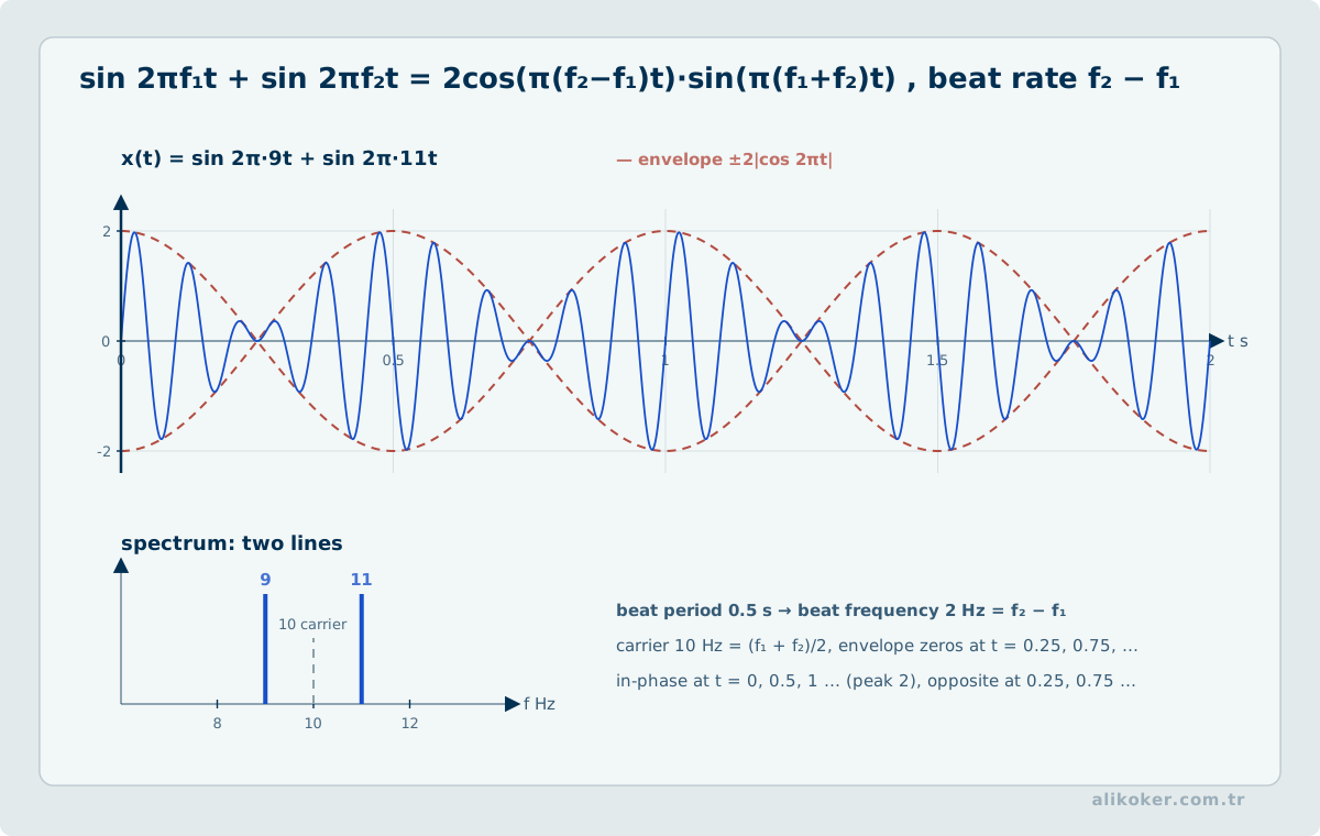
In discrete time:

δ[n] = u[n] - u[n-1]
u[n] = Σ(k=-∞..n) δ[k]

In continuous time the Dirac impulse is defined by its action under integration:

u(t) = ∫(-∞..t)δ(τ)dτ
δ(t) = du(t)/dt
∫x(t)δ(t-t0)dt = x(t0)

The complex exponential,

e^(jωt) = cos(ωt) + j sin(ωt)

is the natural basis for sinusoidal analysis. Continuous-time e^(jω0t) is periodic for every nonzero ω0; discrete-time e^(jω0n) is periodic only when ω0/(2π) is rational, and discrete frequency itself is 2π periodic.

Energy:

E = ∫|x(t)|²dt
E = Σ|x[n]|²

classifies finite-energy signals; periodic signals instead have infinite energy but finite nonzero average power.

Time transformations

x(t-t0)   shift
x(-t)     reversal
x(at)     scaling

Continuous-time scaling is arbitrary; discrete-time indices must remain integral, so rate change is treated as sample removal or insertion.

Even and odd parts are:

x_e(t)=[x(t)+x(-t)]/2
x_o(t)=[x(t)-x(-t)]/2

LTI systems and convolution

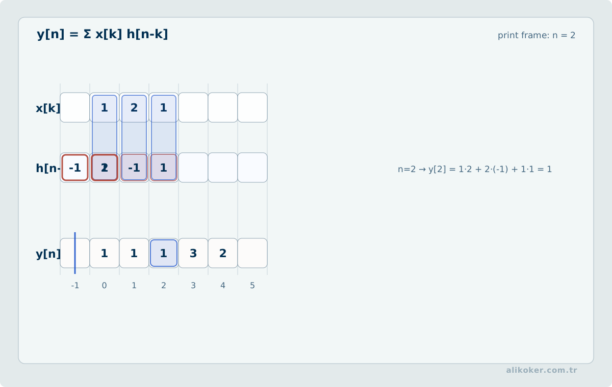
A linear time-invariant system is completely determined by its impulse response.

Discrete time:

x[n]=Σx[k]δ[n-k]
y[n]=Σx[k]h[n-k]=x[n]*h[n]

Continuous time:

y(t)=∫x(τ)h(t-τ)dτ=x(t)*h(t)

Convolution is commutative, associative, and distributive; cascaded LTI systems convolve impulse responses and parallel systems add them.

System properties follow from h:

memoryless   h(t)=Kδ(t)
causal       h(t)=0, t<0
stable       ∫|h(t)|dt < ∞

with Σ|h[n]|<∞ in discrete time.

Step and impulse responses satisfy:

s(t)=u(t)*h(t)
h(t)=ds(t)/dt
h[n]=s[n]-s[n-1]

Differential and difference equations

A continuous LTI system can be written:

Σa_k d^k y(t)/dt^k = Σb_k d^k x(t)/dt^k

and a discrete system:

Σa_k y[n-k] = Σb_k x[n-k]

Initial conditions determine the natural response. Recursive discrete systems generally produce IIR behavior; finite nonrecursive sums produce FIR behavior.

Eigenfunctions and frequency response

Complex exponentials are LTI eigenfunctions:

e^(st) -> H(s)e^(st)
z^n    -> H(z)z^n

The system preserves their form and changes only a scalar coefficient, so H(jω) directly describes sinusoidal amplitude and phase change.

Unit 2: Fourier Analysis and the Frequency Domain

Fourier series

For period T0 and ω0=2π/T0:

x(t)=Σa_k e^(jkω0t)
a_k=(1/T0)∫(T0)x(t)e^(-jkω0t)dt

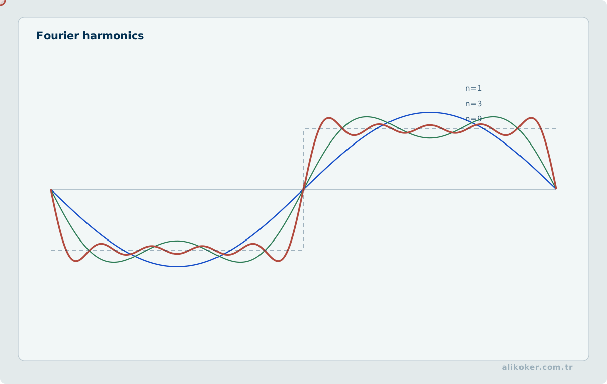
a0 is the average value and real signals have conjugate-symmetric coefficients. Under the Dirichlet conditions, the series converges to the signal at continuity points and to the average of one-sided limits at jumps.

Truncation leaves an overshoot of roughly nine percent near a discontinuity; increasing the number of terms narrows but does not remove it. This is the Gibbs phenomenon.

Parseval:

(1/T0)∫|x(t)|²dt = Σ|a_k|²

connects time-domain average power to harmonic power. A periodic discrete-time sequence has only N distinct harmonics.

Fourier transform

For an aperiodic signal:

X(jω)=∫x(t)e^(-jωt)dt
x(t)=(1/2π)∫X(jω)e^(jωt)dω

Core properties are:

x(t-t0)     <-> e^(-jωt0)X(jω)
dx/dt       <-> jωX(jω)
x(at)       <-> (1/|a|)X(jω/a)
x*h         <-> XH
xh          <-> (1/2π)X*H

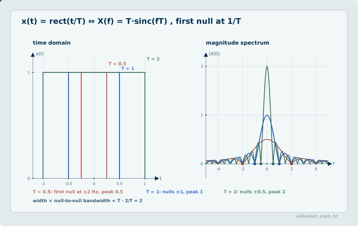
Compression in time expands frequency. Perfect time limitation and perfect band limitation cannot hold simultaneously.

Useful pairs include:

δ(t)          <-> 1
1             <-> 2πδ(ω)
e^(-at)u(t)   <-> 1/(a+jω)
rectangle     <-> sinc

Convolution becoming multiplication is the central simplification of LTI analysis.

DTFT, DFT, and FFT

The DTFT:

X(e^(jω))=Σx[n]e^(-jωn)
x[n]=(1/2π)∫(2π)X(e^(jω))e^(jωn)dω

is 2π periodic.

For N finite samples, the DFT is:

X[k]=Σ(n=0..N-1)x[n]e^(-j2πkn/N)
x[n]=(1/N)Σ(k=0..N-1)X[k]e^(j2πkn/N)

The DFT treats the block as periodic; endpoint mismatch produces spectral leakage.

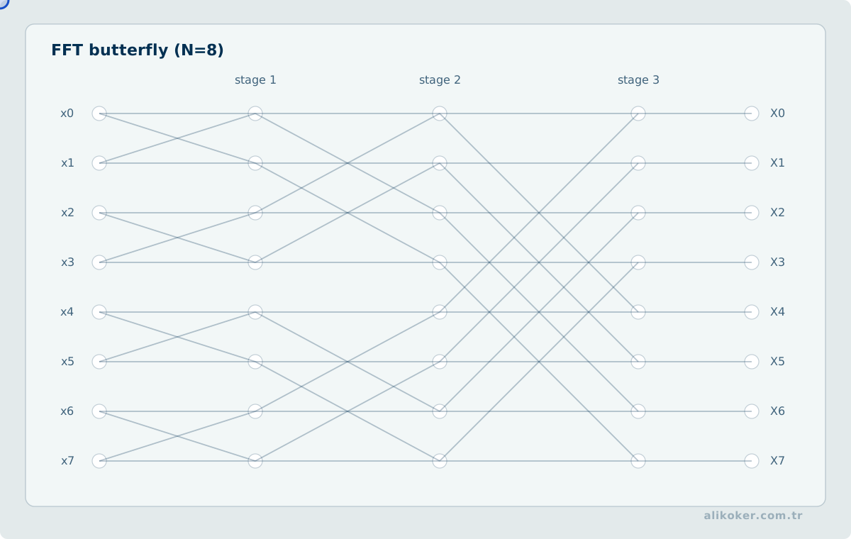
The FFT is not another transform but a family of efficient DFT algorithms. Direct DFT costs about N² operations, while FFT methods require about N log N.

Windowing

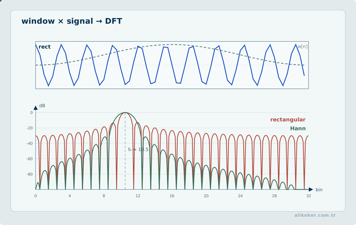
Finite observation multiplies a signal by a window. A rectangular window gives a narrow main lobe but high sidelobes; Hann and Hamming reduce leakage, while Blackman suppresses sidelobes further at the cost of a wider main lobe.

Zero padding samples the displayed spectrum more densely but does not create true frequency resolution; observation duration remains the main limit.

STFT

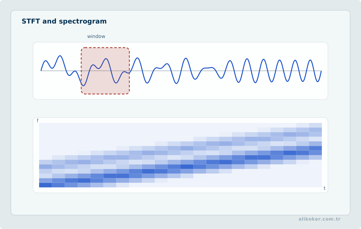
A single Fourier transform gives frequency but not time. The short-time Fourier transform analyzes overlapping windows:

STFT -> spectrogram

Short windows improve time resolution and long windows improve frequency resolution. Speech, music, vibration, radar, and sonar analysis all expose this tradeoff.

Correlation and power spectrum

Cross-correlation,

r_xy[k]=Σx[n]y*[n-k]

measures similarity versus delay; autocorrelation compares a signal with shifted copies of itself. Delay estimation, periodicity detection, matched filtering, and synchronization use the same operation.

The Wiener-Khinchin relation connects autocorrelation and power spectral density. A finite-record periodogram has high variance; Welch's method averages windowed overlapping segments to reduce variance at the cost of frequency resolution.

From the short-time Fourier transform to speech features

A Fourier transform describes the overall frequency content of a record, but speech and many real signals change over time. If a signal is treated as approximately stationary over a short interval, it can be divided into overlapping frames and analyzed separately. The short-time Fourier transform (STFT) builds this time-frequency representation.

samples
→ framing
→ windowing
→ STFT
→ time-frequency coefficients
→ spectrogram

Frame length and hop size are chosen together. Short frames track rapid change more closely but provide poorer frequency discrimination; longer frames improve frequency discrimination while reducing time localization. Windowing helps control spectral leakage created by finite frame boundaries.

In speech processing, the STFT is often the beginning rather than the final feature representation. A common chain is:

STFT
→ power spectrum
→ Mel filter bank
→ log energy
→ log-Mel representation

The Mel scale samples frequency with a resolution closer to human auditory perception, while the logarithm compresses a wide energy range. A further transform can produce cepstral coefficients. The full path is discussed in Speech Feature Extraction with MFCC and From Spectrum to Cepstrum in Audio Processing.

Feature representations must also be kept distinct from quality metrics. SNR concerns signal and noise energy; PESQ and STOI concern perceived speech quality or intelligibility. WER and CER measure errors in the text produced by a speech recognizer. Good signal quality does not guarantee low WER, and WER alone does not describe the perceptual quality of enhanced audio.

Similarly, voice activity detection (VAD) is primarily a segmentation problem: it estimates where speech is active. MFCC or log-Mel features represent selected intervals numerically. Modern recognizers may combine or internalize these stages in different ways. Whisper Architecture in Speech Recognition Systems provides a separate end-to-end example.

The engineering lesson is that every transformation between waveform samples and model input preserves, emphasizes, or discards information. Feature extraction should therefore be understood as controlled representation of signal information, not merely as tensor preparation.

From spectrum to cepstrum, MFCC, and ASR model input

The time-frequency representation produced by the STFT is only the first transformation in a speech-processing chain. Taking the logarithm of spectral power converts multiplicative spectral structure into an additive form; a second transform of the log spectrum produces a cepstral coordinate system. In the real cepstrum that second transform is commonly an inverse Fourier transform. In an MFCC pipeline, spectral energy is first accumulated by a Mel filter bank, mapped to the log domain, and then usually transformed with a DCT. MFCC and the directly computed real cepstrum are therefore not the same object; their shared idea is to represent log-spectral structure with coefficients that are easier to separate and compress (Davis and Mermelstein, 1980; Oppenheim and Schafer, 2004).

This distinction matters when interpreting model input. Classical recognizers widely used hand-designed features such as MFCC, whereas some modern systems feed a log-Mel spectrogram directly to a neural network. Whisper is a clear example (Radford et al., 2022). Saying that a model does not use an explicit cepstrum therefore does not mean that Fourier analysis or log-spectral representation has become irrelevant; part of the transformation chain has simply moved before or inside the learned model.

The application path is developed at different layers in From Spectrum to Cepstrum in Audio Processing, Speech Feature Extraction with MFCC, and Whisper Architecture in Speech Recognition Systems. The co-authored Image and Audio Processing — Book Chapter brings audio feature vectors, speech recognition, and speaker recognition together in one published work. That link provides author provenance for the application context; the general claims about Fourier analysis, cepstrum, and MFCC remain grounded in independent academic sources.

Autocorrelation and power spectral density

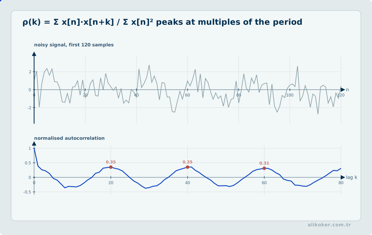
Autocorrelation measures similarity between a signal and delayed versions of itself as a function of lag. For a wide-sense stationary process it can be written conceptually as

R_xx(tau) = E[x(t) x(t+tau)].

Under suitable conditions, the Wiener-Khinchin relation connects power spectral density to the Fourier transform of the autocorrelation. Time-domain lag structure and frequency-domain power distribution are therefore two views of the same second-order information.

A periodogram computed from a finite record is an estimate rather than the exact PSD. Window choice, segment length, and averaging create a resolution-versus-variance trade-off.

Unit 3: Sampling, Multirate Processing, and Filters

Sampling and quantization

Impulse-train sampling:

x_p(t)=x(t)Σδ(t-nT)

replicates the spectrum at ωs=2π/T intervals:

X_p(jω)=(1/T)ΣX(j(ω-kωs))

For bandlimit ωM, the condition ωs>2ωM keeps replicas separate. 2ωM is the Nyquist rate, not the selected physical sample rate.

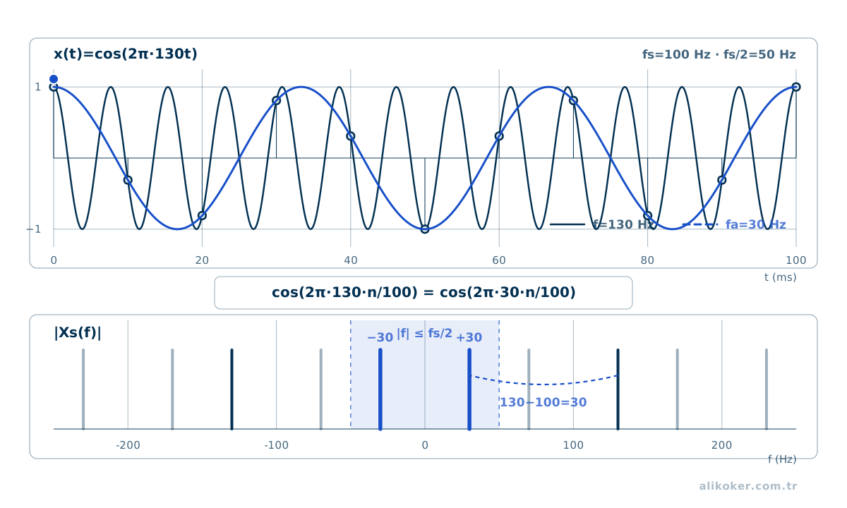
Aliasing makes high-frequency components appear at lower frequencies and destroys information at sampling time. A practical ADC chain is therefore:

analog -> anti-alias filter -> sample/hold -> ADC -> digital data

Sampling discretizes time; quantization discretizes amplitude. An ideal B-bit ADC has 2^B levels and roughly:

SNR ≈ 6.02B + 1.76 dB

for a full-scale sinusoid. Thermal noise, clock jitter, and nonlinearity reduce practical ENOB.

Ideal reconstruction uses sinc interpolation; practical DACs use a zero-order hold followed by an analog reconstruction filter.

Multirate processing

Downsampling requires:

low-pass -> keep every Mth sample

and interpolation requires:

insert L-1 zeros -> low-pass

Without prefiltering, decimation aliases the discrete spectrum. Rational L/M conversion combines both operations; polyphase structures avoid computations that would later be discarded.

Filters

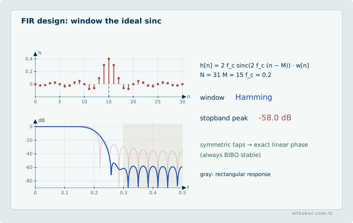
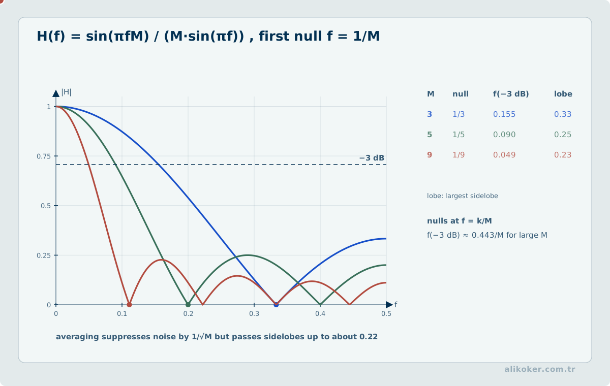
The main responses are low-pass, high-pass, band-pass, band-stop, and all-pass. A brick-wall response is noncausal, so real filters trade transition width, ripple, attenuation, phase, order, and computation.

FIR:

y[n]=Σb_k x[n-k]

is finite, nonrecursive, always BIBO stable, and can have exact linear phase.

IIR:

y[n]=-Σa_k y[n-k]+Σb_k x[n-k]

can reach a given selectivity with fewer coefficients but requires pole-stability and numerical-sensitivity analysis.

Classical families include Butterworth, Chebyshev I and II, elliptic, and Bessel filters, each choosing a different balance among flatness, transition sharpness, and phase behavior.

Phase and group delay

Distortionless transmission requires:

H(jω)=Ke^(-jωt0)

so magnitude is constant and phase is linear.

Group delay:

τg(ω)=-d∠H(jω)/dω

describes narrowband envelope delay. Frequency-dependent group delay spreads pulses and may distort communication symbols.

Bode magnitude uses:

20log10|H(jω)|

so cascade gains become sums in dB.

Resampling, interpolation, and sample-rate conversion

Changing the sampling rate of a discrete signal is not merely dropping indices or inserting zeros. After upsampling, an interpolation filter suppresses spectral images. Before downsampling, an anti-alias filter suppresses content above the new Nyquist limit.

For a rational conversion ratio

L / M,

the conceptual chain is upsample by L, apply an appropriate low-pass filter, and downsample by M. Polyphase implementations avoid many unnecessary operations.

This appears in audio sample-rate conversion, sensor fusion, and alignment of streams with different time bases. General interpolation theory belongs to Numerical Analysis; here the focus is band-limited signals and aliasing.

Unit 4: Laplace, z Transform, and State Space

Laplace transform

X(s)=∫x(t)e^(-st)dt
s=σ+jω

extends Fourier analysis with exponential weighting and a region of convergence. The ROC is part of the transform because the same algebraic expression can represent different time-domain signals under different ROCs.

For a causal rational system, the ROC lies to the right of the rightmost pole; stability requires the jω axis to lie inside the ROC. A causal stable continuous-time rational system therefore has all poles in the left half-plane.

The system function:

H(s)=Y(s)/X(s)

comes directly from the differential equation under initial rest. The unilateral transform includes initial conditions:

L{dx/dt}=sX(s)-x(0-)

z transform

The discrete-time counterpart is:

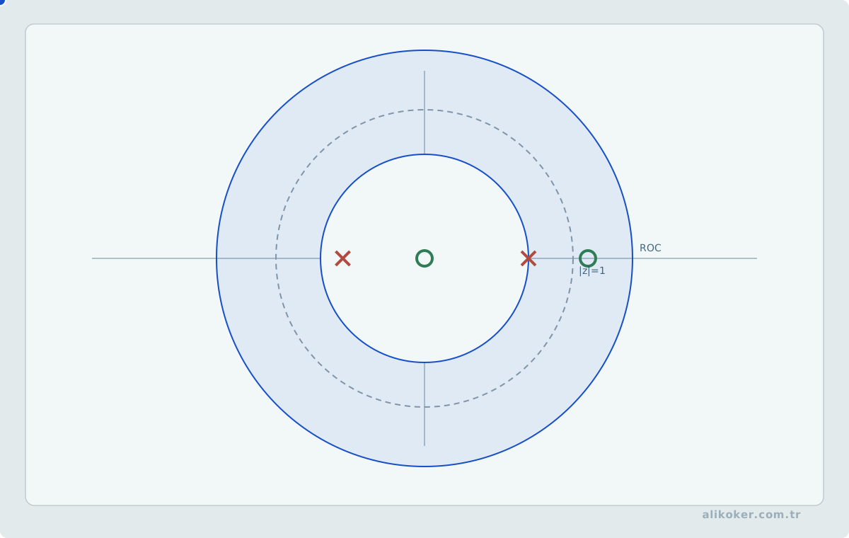
X(z)=Σx[n]z^(-n)

and the unit circle corresponds to the DTFT.

For a causal rational discrete-time system, the ROC lies outside the outermost pole; stability requires the unit circle to lie inside the ROC. A causal stable system therefore has all poles inside the unit circle.

Difference equations produce:

H(z)=B(z)/A(z)

and poles near the unit circle create longer memory and sharper frequency selectivity.

Numerical realization

A high-order IIR implemented as one polynomial is numerically fragile; cascaded second-order sections are usually more robust:

H(z)=H1(z)H2(z)...Hm(z)

Overflow, rounding, coefficient quantization, and limit cycles are system effects in finite-precision implementations. Direct, cascade, and parallel realizations of the same theoretical transfer function can behave differently.

State space

A transfer function describes input-output behavior; state space exposes internal memory.

Continuous time:

x_dot=Ax+Bu
y=Cx+Du

Discrete time:

x[n+1]=Ax[n]+Bu[n]
y[n]=Cx[n]+Du[n]

The state is the smallest internal information set needed to predict future behavior given future input. MIMO systems, controllability, and observability are naturally expressed in this form.

Controllability, observability, and the bridge to Kalman filtering

For a state-space model

x_(k+1) = A x_k + B u_k
y_k     = C x_k + D u_k,

controllability asks whether suitable inputs can drive the state through the required directions, while observability asks whether the internal state can be distinguished from output history.

These are relevant not only to control but also to state estimation. In a linear-Gaussian setting, the Kalman filter recursively combines model prediction with measurement information using uncertainty covariances.

The goal here is not to derive every Kalman equation. It is to place the filter in the correct context of state space, noise models, and observability rather than treating it as a generic smoothing routine. Its statistical interpretation connects to conditional Gaussian models in Probability and Statistics.

Unit 5: Communications, Feedback, and Real Processing Chains

Modulation and communications

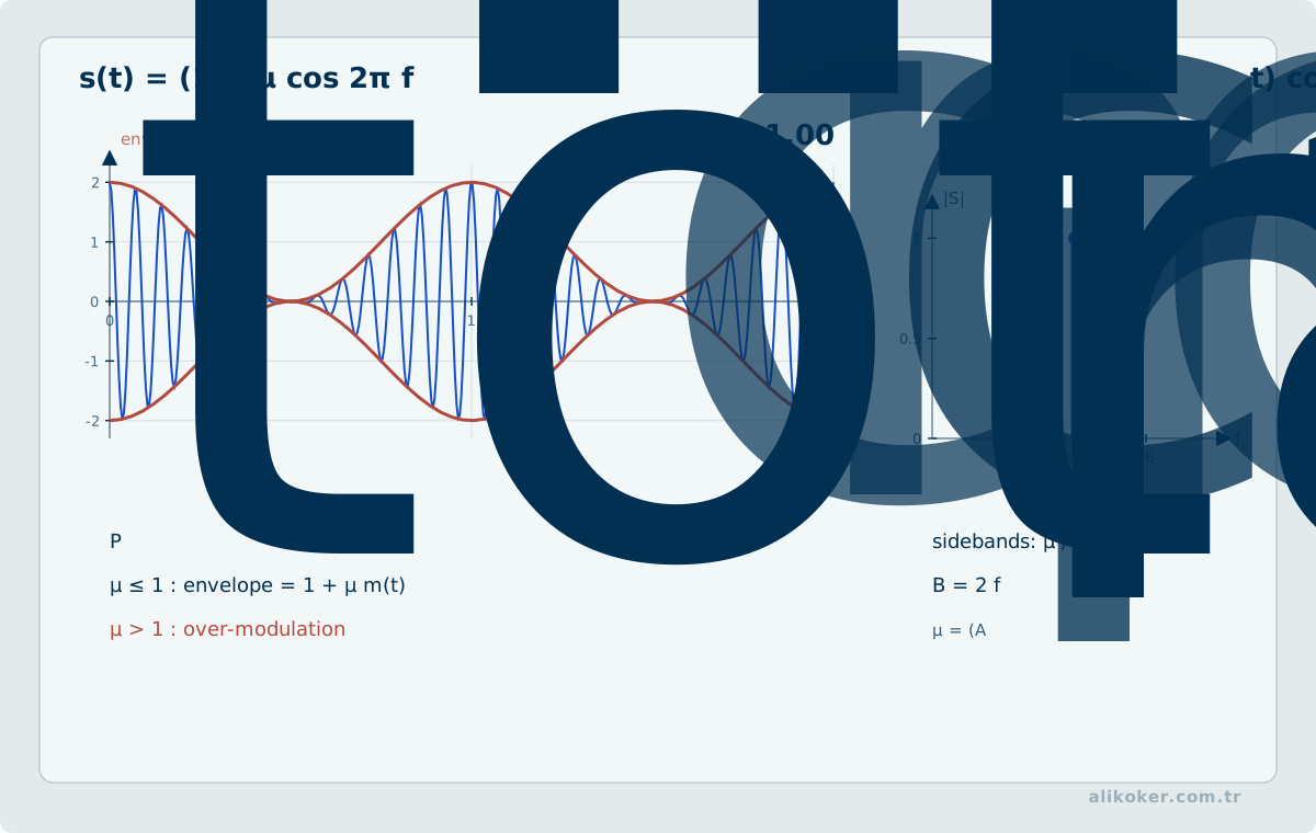
Amplitude modulation follows:

x(t)cos(ωct)
<->
(1/2)[X(j(ω-ωc))+X(j(ω+ωc))]

Coherent detection needs carrier phase; envelope detection simplifies the receiver at the cost of carrier power. Single-sideband transmission carries the same information in half the DSB bandwidth.

Frequency modulation places information in instantaneous frequency and trades more bandwidth for improved tolerance to amplitude noise.

PAM carries symbol amplitudes, while QAM uses two quadrature carrier components. Band limitation causes intersymbol interference; raised-cosine and root-raised-cosine pulse shaping balance bandwidth and timing robustness.

OFDM divides data among many orthogonal subcarriers implemented efficiently with the DFT/FFT. A cyclic prefix simplifies multipath equalization, while peak-to-average power ratio, carrier-frequency error, and prefix overhead remain its main costs.

Matched filter

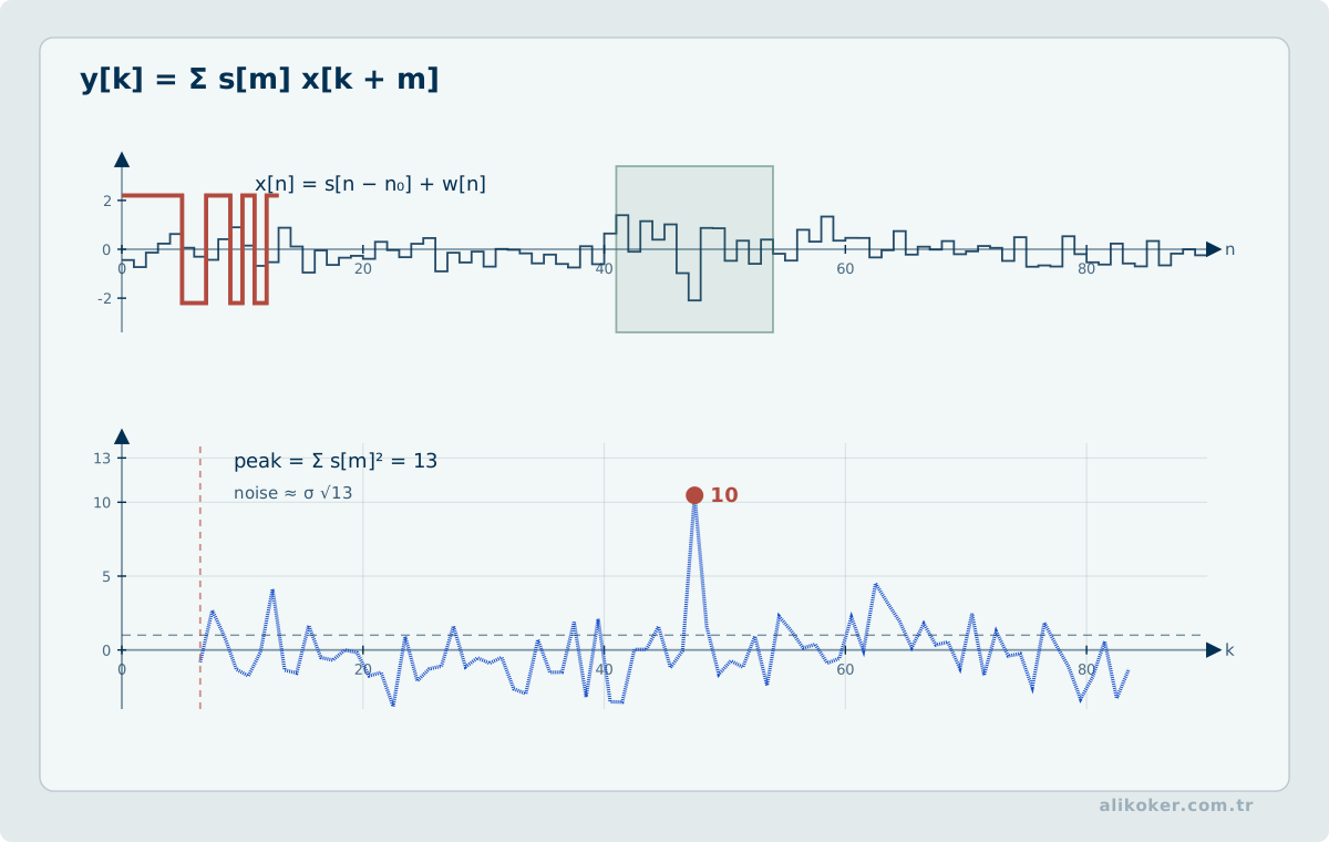
For a known waveform in white noise, the LTI filter that maximizes SNR at the chosen sampling instant is the matched filter; its impulse response is proportional to the time-reversed conjugate of the target waveform. Radar, sonar, digital communications, and correlation-based detection all use this result.

Feedback

Negative feedback gives:

Q=H1/(1+H1H2)

with closed-loop poles satisfying 1+H1H2=0.

Feedback can reduce sensitivity and disturbances, improve tracking, and stabilize an unstable plant; unfavorable phase can also destabilize an otherwise stable system.

Root locus shows pole motion with gain. The Nyquist criterion relates encirclements of -1 to closed-loop stability. Gain and phase margins measure distance to instability; pure delay changes no magnitude but consumes phase margin.

Real processing chains

Separate theory topics merge in real systems:

physical source
-> analog front end
-> anti-alias filter
-> ADC
-> buffer
-> digital filter
-> transform / feature
-> decision / coding
-> transmission / storage

For real-time work, latency, block size, computational cost, memory access, numerical precision, clock drift, and sample loss matter alongside mathematical correctness. Longer FFTs refine frequency spacing but increase block latency; longer FIR filters sharpen transitions but increase computation and group delay.

One framework

time domain          transform domain
------------------   ----------------
convolution          multiplication
derivative/difference frequency weighting
shift                phase factor
exponential input    scalar gain
stability            poles + ROC

Fourier series decomposes periodic signals into harmonics, Fourier transform describes aperiodic spectra, Laplace adds the continuous-time ROC, and the z transform adds the discrete-time ROC.

The continuous-time stability boundary is the jω axis and the discrete-time boundary is the unit circle; sampling connects their frequencies through ω=ΩT.

Key distinctions

• Linearity requires zero input to produce zero output.
• Real-time physical operation requires causality; offline processing may be noncausal.
• BIBO stability requires an absolutely integrable or summable impulse response.
• A discrete sinusoid is periodic only when normalized frequency is rational.
• DTFT has a continuous periodic frequency variable; DFT has finitely many frequency samples.
• FFT is a DFT algorithm, not a new transform.
• Zero padding does not create true frequency resolution.
• Sampling discretizes time; quantization discretizes amplitude.
• The Nyquist rate is a lower bound, not the chosen sampling rate.
• Aliasing is irreversible information loss.
• Decimation requires prior band limitation.
• FIR is finite and nonrecursive; IIR requires pole-stability analysis.
• Linear phase is not zero phase.
• Laplace and z transforms are incomplete without their ROCs.
• Causal stable continuous-time poles lie in the left half-plane; discrete-time poles lie inside the unit circle.
• Finite-precision realizations of the same transfer function can behave differently.
• Open-loop stability alone does not determine closed-loop stability.

Sampling, aliasing, and windowing

Sampling theory is more than choosing a rate above twice one frequency. Real signals are rarely perfectly band-limited, so an anti-alias filter must attenuate energy outside the intended band before the ADC.

An FFT of a finite record also includes the spectral effect of the window. Signals that do not align with FFT bins exhibit leakage, and window choice trades main-lobe width against sidelobe suppression.

Amplitude and noise measurements should account for coherent gain and equivalent noise bandwidth so the spectrum becomes a quantitative instrument rather than just a plot.

Scale and sampling conditions in signal analysis

An FFT plot is incomplete without record length and sample rate. Frequency resolution, window choice, zero-padding, and amplitude scaling all affect interpretation. Zero-padding does not add spectral information; it only samples the displayed frequency axis more densely.

For LTI systems, time- and frequency-domain solutions can cross-check each other. Convolution and transfer-function methods should agree under the same assumptions.

Physical measurement also includes anti-alias filtering and sensor bandwidth. Checking the Nyquist condition only from the digital sample rate ignores the analog content reaching the ADC.

The Interaction Between Signal Processing and Artificial Intelligence

The relationship between signal processing and AI is bidirectional. Signal processing turns a physical measurement into a sampled, meaningful representation; learning methods use those representations for classification, estimation, separation, or reconstruction. Learned front ends can replace some hand-designed features, but they do not remove sampling theory or measurement physics.

From physical signal to model input

Audio, vibration, and communication signals must be measured and sampled. If the Nyquist condition is violated, aliasing folds distinct frequency components together. A larger neural network cannot deterministically reconstruct information that was never sampled correctly.

physical signal
↓
sampling
↓
digital representation
↓
time / frequency / time-frequency transform
↓
learning model

Fourier and time-frequency representation

Speech and many acoustic events are nonstationary. A single Fourier transform of an entire recording hides temporal evolution. STFT exposes local spectra through windows. Window length and hop size trade time resolution against frequency resolution.

If a model consumes spectrograms, sample rate, window, hop, scaling, and normalization are part of the model contract. Training with one front end and serving with another can create distribution shift even when tensor dimensions match.

Hand-designed and learned features

Classical speech systems often use MFCCs, filter-bank energies, or other engineered features. Modern neural systems may learn representations from waveforms or lower-level features. The distinction is:

classical: signal → designed feature → classifier
learned:   signal → learned representation → decision

Hybrid designs are common; log-Mel features can encode useful signal knowledge while later representations are learned.

Two meanings of convolution

For an LTI system:

y[n] = Σ x[k] h[n-k]

where h is the impulse response. A convolutional neural network uses a similar sliding operation, but a learned kernel is not necessarily a physical impulse response. The operator is related; the modeling interpretation is different.

Noise, augmentation, and robustness

Physical noise and data augmentation are not the same. Augmentation is an imposed training distribution. If it does not represent field conditions, it can optimize the model for the wrong problem. SNR, clipping, reverberation, and channel effects should be tied to the actual operating environment.

What learning adds

Denoising, source separation, speech recognition, acoustic-event detection, and channel estimation can benefit from learned high-dimensional mappings. Yet the output of a learned enhancement model is an estimate, not the original physical signal. In forensic or measurement contexts that distinction is essential.

Evaluation should therefore remain layered:

measurement → SNR / clipping / sampling
signal transform → spectral or waveform error
model task → WER / accuracy / F1 / task metric
system → latency / RTF / throughput

Improvement at one layer does not guarantee improvement at another.

Signal processing is not merely preprocessing for AI, and AI is not an automatic replacement for DSP. Signal processing determines what information is represented from the physical world; learning determines what task-relevant mapping can be estimated from that representation.

Choosing the Representation Domain for the Problem

The transforms used in Signals and Systems express the same signal in different mathematical languages. The time domain shows when samples or events occur and with what amplitude; the frequency domain makes the spectral components of variation explicit. For a linear time-invariant system, convolution in time becomes multiplication in frequency. A long convolution calculation can therefore become the simpler relation Y(f) = X(f)H(f). If the question concerns switching time, delay, or the temporal structure of an impulse response, the time domain may instead be the clearer representation.

A Fourier series represents a periodic signal by discrete harmonics, whereas the Fourier transform provides a continuous-frequency representation for signals that need not be periodic. The Laplace transform extends frequency reasoning into the complex plane so that growth and decay are represented explicitly; its region of convergence is therefore part of the mathematical meaning rather than a bookkeeping detail. For discrete-time systems, the z-transform plays a comparable role, and pole locations relative to the unit circle connect directly to stability.

The most important sampling distinction is that a high sampling rate cannot repair every mistake after the fact. The Nyquist condition is a reconstruction condition for a signal assumed to be band-limited before sampling. Once distinct spectral components have folded onto one another through aliasing, a later digital filter cannot in general recover the lost distinction.

Before selecting a transform, identify whether the signal is continuous or discrete, periodic or aperiodic, whether the system satisfies the LTI assumptions, and which information the problem asks you to preserve. Fourier, Laplace, and z-domain methods are then not competing formulas but complementary representations of system behaviour under different assumptions.

Advanced Extension: Outliers and Robust Feature Extraction in Signal Measurement

Robust statistics asks how much an estimator degrades under small departures from an idealized model. Beyond robust summaries such as the median and MAD, the influence function and breakdown point provide more formal descriptions of sensitivity to contaminated observations. In heavy-tailed or contaminated data, decisions based only on the mean and standard deviation can be misleading.

In the context of Signals and Systems, this perspective can be made concrete in the following ways:

• Show how mean-based features degrade under impulsive noise.
• State which corruption modes benefit from median-based filtering or summaries.
• Preserve the distinction between suppressing anomalies and deleting genuine transients.

The purpose of this extension is not to replace the existing fundamentals, but to make explicit the measurement and correctness boundaries that appear in high-volume, concurrent, or fault-tolerant systems. An optimization should not be treated as established without measurement, a relationship metric should not be treated as causal evidence, and an approximate algorithm should not be treated as exact without an explicit error bound.

Conceptual source basis: Peter J. Huber; Elvezio M. Ronchetti — Robust Statistics; Mor Harchol-Balter — Performance Modeling and Design of Computer Systems.

References

• Alan V. Oppenheim; Ronald W. Schafer. (2004). From Frequency to Quefrency: A History of the Cepstrum. IEEE Signal Processing Magazine, 21(5), 95-106. doi:10.1109/MSP.2004.1328092

• Alec Radford; Jong Wook Kim; Tao Xu; Greg Brockman; Christine McLeavey; Ilya Sutskever. (2022). Robust Speech Recognition via Large-Scale Weak Supervision. arXiv. doi:10.48550/arXiv.2212.04356

• Alex Graves, Abdel-rahman Mohamed, Geoffrey Hinton. “Speech Recognition with Deep Recurrent Neural Networks.” ICASSP, 2013. https://doi.org/10.1109/ICASSP.2013.6638947

• Cooley, J. W., & Tukey, J. W. “An Algorithm for the Machine Calculation of Complex Fourier Series.” Mathematics of Computation, 19(90), 1965. https://doi.org/10.1090/S0025-5718-1965-0178586-1

• Franklin, G. F., Powell, J. D., & Emami-Naeini, A. Feedback Control of Dynamic Systems, 8th ed. Pearson, 2019.

• Geoffrey Hinton et al. “Deep Neural Networks for Acoustic Modeling in Speech Recognition.” IEEE Signal Processing Magazine, 29(6), 2012. https://doi.org/10.1109/MSP.2012.2205597

• Harris, F. J. “On the Use of Windows for Harmonic Analysis with the Discrete Fourier Transform.” Proceedings of the IEEE, 66(1), 1978. https://doi.org/10.1109/PROC.1978.10837

• Haykin, S., & Van Veen, B. Signals and Systems, 2nd ed. Wiley, 2003.

• Lathi, B. P. Linear Systems and Signals, 2nd ed. Oxford University Press, 2005.

• Lyons, R. G. Understanding Digital Signal Processing, 3rd ed. Pearson, 2011.

• Oppenheim, A. V., & Schafer, R. W. Discrete-Time Signal Processing, 3rd ed. Pearson, 2010.

• Oppenheim, A. V., Willsky, A. S., & Nawab, S. H. Signals and Systems, 2nd ed. Prentice Hall, 1997.

• Proakis, J. G., & Manolakis, D. G. Digital Signal Processing: Principles, Algorithms, and Applications, 4th ed. Pearson, 2007.

• Proakis, J. G., & Salehi, M. Digital Communications, 5th ed. McGraw-Hill, 2007.

• Shannon, C. E. “Communication in the Presence of Noise.” Proceedings of the IRE, 37(1), 1949. https://doi.org/10.1109/JRPROC.1949.232969

• Steven Davis; Paul Mermelstein. (1980). Comparison of Parametric Representations for Monosyllabic Word Recognition in Continuously Spoken Sentences. IEEE Transactions on Acoustics, Speech, and Signal Processing, 28(4), 357-366. doi:10.1109/TASSP.1980.1163420

• Welch, P. D. “The Use of Fast Fourier Transform for the Estimation of Power Spectra.” IEEE Transactions on Audio and Electroacoustics, 15(2), 1967. https://doi.org/10.1109/TAU.1967.1161901