Probability and Statistics: Distributions, Sampling and Regression

Unit 1: Introduction to Statistics

Core concepts

Statistics is the set of methods used to collect, organize, analyze, and interpret data.

A population is the complete set of units about which information is sought.

A sample is a subset selected from the population.

A census examines every unit in the population.

Sampling selects a sample from the population according to a defined procedure.

A unit is a single object of observation.

A variable is a measured or classified property of a unit.

A numerical quantity describing a population is a parameter; its sample-based counterpart is a statistic. Statistical inference uses the sample to draw conclusions about the population.

Levels of measurement

• Nominal: identifies categories without an inherent order.
• Ordinal: has an order, but distances between levels are not assumed equal.
• Interval: equal differences are meaningful, but there is no true zero.
• Ratio: has equal intervals and a true zero, so ratios are meaningful.

Encoding a category as 1, 2, or 3 does not make it quantitative. Coding and level of measurement are different concepts.

Interpretation must also respect the level of aggregation. Inferring individual behavior from relationships observed at a regional, organizational, or time-aggregated level is an ecological fallacy.

Descriptive and inferential statistics

Descriptive statistics summarizes the observed data.

Inferential statistics uses a sample to make uncertainty-aware statements about a population.

The distinction is fundamental: a mean and standard deviation describe data; a standard error and confidence interval quantify sampling uncertainty.

Measures of central tendency

Arithmetic mean

x̄ = Σxᵢ / n
x̄ = Σ(fᵢ·xᵢ) / Σfᵢ

For grouped data, xᵢ is the class midpoint.

The arithmetic mean uses every observation and is sensitive to outliers.

Geometric mean

G = ⁿ√(x₁·x₂·...·xₙ)
log G = Σ(log xᵢ) / n

It is appropriate for positive multiplicative changes, growth rates, and compound returns.

Harmonic mean

H = n / Σ(1/xᵢ)

It is useful for averaging rates when the denominator structure requires it.

Root mean square

K = √(Σxᵢ² / n)

It measures magnitude independently of sign.

For positive values:

H ≤ G ≤ x̄ ≤ K

Median

The median is the middle value of an ordered data set. It is more robust to outliers than the mean.

For grouped data:

Md = L + [ (n/2 − F) / f ] · c

L is the lower boundary of the median class, F the cumulative frequency before it, f its frequency, and c the class width.

Mode

The mode is the most frequent value. A distribution may have no mode or multiple modes.

For grouped data:

Mo = L + [ Δ₁ / (Δ₁ + Δ₂) ] · c

For a symmetric unimodal distribution:

x̄ = Md = Mo

Measures of dispersion

Range:

R = x_max − x_min

It depends only on the minimum and maximum and is therefore sensitive to extremes.

Interquartile range:

IQR = Q₃ − Q₁

It measures the spread of the middle 50% and is more robust to outliers.

Population variance:

σ² = Σ(xᵢ − μ)² / N

Sample variance:

s² = Σ(xᵢ − x̄)² / (n − 1)

Standard deviation:

s = √s²

Standard deviation describes the spread of observations. Standard error describes the sampling variability of an estimator.

For independent observations, the estimated standard error of the sample mean is:

SE(x̄) = s / √n

Coefficient of variation:

CV = (s / x̄) · 100

It can compare relative variability of positive ratio-scale quantities. It becomes unstable when the mean is near zero.

Percentiles and quantiles

The median is the 50th percentile. Q₁, Q₂, and Q₃ correspond to the 25th, 50th, and 75th percentiles.

P90, P95, and P99 summarize upper-tail behavior. P95, for example, is a threshold at or below which approximately 95% of observations fall.

Percentile algorithms can differ in rank definition and interpolation, especially in small samples. Comparisons should use the same method.

Robust statistics

When outliers distort the mean and standard deviation, the median and median absolute deviation can provide robust summaries:

MAD = median(|xᵢ − median(x)|)

Modified z-score:

Mᵢ = 0.6745 · (xᵢ − median(x)) / MAD

It is an anomaly indicator, not proof. The expression cannot be applied directly when MAD = 0.

Classical z-score:

zᵢ = (xᵢ − x̄) / s

Unit 2: Set Theory

Sets and subsets

A set is a collection of objects; its objects are elements.

If every element of A belongs to B:

A ⊆ B

A set with n elements has:

2ⁿ

subsets.

Intersection, union, and complement

A ∩ B = {x : x ∈ A and x ∈ B}
A ∪ B = {x : x ∈ A or x ∈ B}
A' = {x ∈ E : x ∉ A}
A \ B = A ∩ B'

De Morgan's laws:

(A ∪ B)' = A' ∩ B'
(A ∩ B)' = A' ∪ B'

Inclusion-exclusion:

|A ∪ B| = |A| + |B| − |A ∩ B|

Set theory provides the language of probability: the sample space is a set and an event is a subset.

Unit 3: Permutations and Combinations

Counting principles

Counts are added for mutually exclusive alternatives and multiplied for successive stages.

Permutations

Order matters:

P(n,r) = n! / (n−r)!
P(n,n) = n!

Sampling with replacement:

nʳ

With identical elements:

n! / (n₁!·n₂!·...·nₖ!)

Combinations

Order does not matter:

C(n,r) = n! / [r!·(n−r)!]

Combinations with repetition:

C(n+r−1,r)

Properties:

C(n,r) = C(n,n−r)
C(n,r) = C(n−1,r−1) + C(n−1,r)
Σ C(n,r) = 2ⁿ

If changing order changes the outcome, use a permutation; otherwise use a combination.

Unit 4: Introduction to Probability

Basic concepts

A random experiment has an outcome that cannot be known with certainty in advance. The set of all possible outcomes is the sample space. A subset of the sample space is an event.

Definitions of probability

For equally likely outcomes:

P(A) = favorable outcomes / possible outcomes

In the frequentist view, probability is the limiting relative frequency under repeated trials.

Kolmogorov axioms:

0 ≤ P(A) ≤ 1
P(S) = 1
If A and B are disjoint:
P(A ∪ B) = P(A) + P(B)

Basic results:

P(∅) = 0
P(A') = 1 − P(A)
P(A ∪ B) = P(A) + P(B) − P(A ∩ B)

For three events:

P(A∪B∪C)
= P(A)+P(B)+P(C)
− P(A∩B)−P(A∩C)−P(B∩C)
+ P(A∩B∩C)

Conditional probability

P(A|B) = P(A ∩ B) / P(B),   P(B) > 0

Multiplication rule:

P(A ∩ B) = P(B)·P(A|B)
         = P(A)·P(B|A)

Independence

P(A|B) = P(A)

equivalently:

P(A ∩ B) = P(A)·P(B)

Disjointness is not independence. Two disjoint events with nonzero probabilities cannot be independent.

Law of total probability

If B₁, ..., Bₙ partition the sample space:

P(A) = ΣP(Bᵢ)·P(A|Bᵢ)

Bayes' theorem

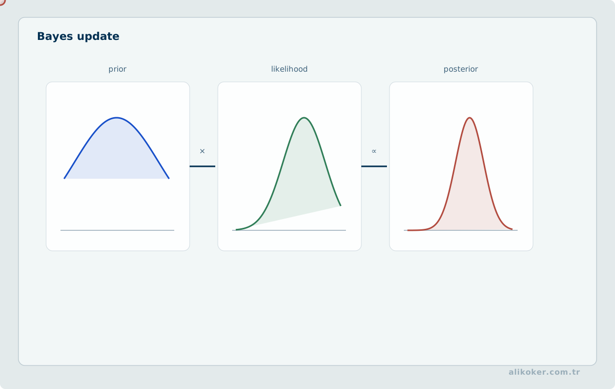
P(Bₖ|A)
= P(Bₖ)·P(A|Bₖ) / Σ[P(Bᵢ)·P(A|Bᵢ)]

P(Bₖ) is the prior probability and P(Bₖ|A) the posterior probability. New evidence updates prior information.

Unit 5: Random Variables

Discrete and continuous variables

A discrete random variable takes countable values.

A continuous random variable can take values across an interval.

Discrete distributions

p(xᵢ) = P(X = xᵢ)
p(xᵢ) ≥ 0
Σp(xᵢ) = 1

Cumulative distribution:

F(x) = P(X ≤ x)

Expected value:

E(X) = μ = Σxᵢ·p(xᵢ)

Variance:

Var(X) = E[(X−μ)²]
       = E(X²) − [E(X)]²

Properties:

E(aX+b) = aE(X)+b
E(X+Y) = E(X)+E(Y)
Var(aX+b) = a²Var(X)

In general:

Var(X+Y)
= Var(X)+Var(Y)+2Cov(X,Y)

Continuous distributions

Probability density function:

f(x) ≥ 0
∫f(x)dx = 1
P(a ≤ X ≤ b) = ∫[a,b] f(x)dx

For a continuous distribution, a single point has probability zero.

F(x) = ∫(−∞,x] f(t)dt
E(X) = ∫x·f(x)dx
Var(X) = ∫(x−μ)²f(x)dx

Unit 6: Discrete Probability Distributions

Bernoulli distribution

A single trial with two outcomes:

P(X=1) = p
P(X=0) = 1−p = q
E(X) = p
Var(X) = p·q

Binomial distribution

Number of successes in n independent Bernoulli trials:

P(X=k) = C(n,k)·pᵏ·q^(n−k)
E(X) = n·p
Var(X) = n·p·q

The model requires a fixed number of trials, two outcomes per trial, constant success probability, and independent trials.

Multinomial distribution

An extension of the binomial model to more than two outcomes:

P(X₁=n₁,...,Xₖ=nₖ)
= [n!/(n₁!·...·nₖ!)] · p₁^n₁ · ... · pₖ^nₖ

Poisson distribution

Models the number of events in a fixed time or spatial interval:

P(X=k) = e^(−λ)·λᵏ/k!
E(X) = λ
Var(X) = λ

Under the theoretical Poisson model, mean and variance are equal. Strong overdispersion or underdispersion in observed data calls model adequacy into question.

A Poisson approximation to the binomial is appropriate when n grows, p becomes small, and λ=n·p remains bounded. Fixed numerical cutoffs are only rules of thumb.

Geometric distribution

Number of trials until the first success:

P(X=k) = q^(k−1)·p
E(X) = 1/p

It is memoryless.

Negative binomial distribution

Models the number of trials until the rth success. The geometric distribution is the special case r=1.

Unit 7: Continuous Probability Distributions

Normal distribution

f(x)
= [1/(σ√(2π))]
  · e^(−(x−μ)²/(2σ²))

μ determines location and σ dispersion.

Properties:

• symmetric about μ;
• mean, median, and mode coincide;
• total area under the curve is 1;
• inflection points occur at μ ± σ.

Approximate empirical rule:

μ ± σ   → 68%
μ ± 2σ  → 95%
μ ± 3σ  → 99.7%

Standard normal distribution

Z = (X−μ)/σ

Z expresses how many standard deviations an observation lies from the mean.

Central limit theorem

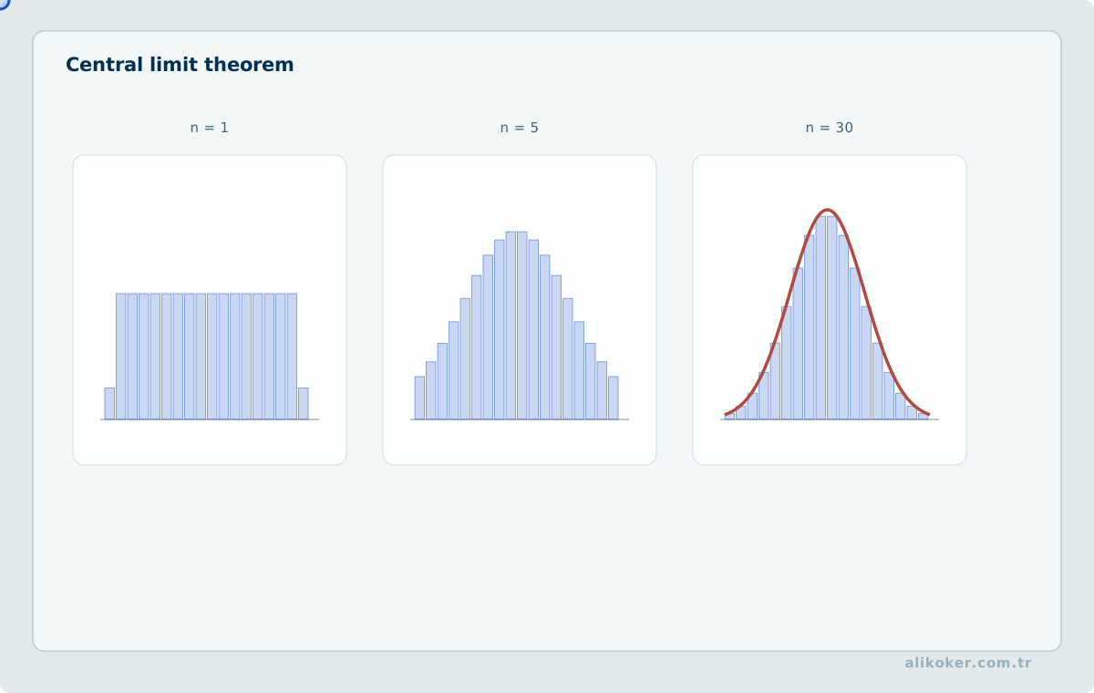
Under suitable independence and regularity conditions, the standardized distribution of the sample mean approaches normality as sample size grows:

X̄ ≈ N(μ, σ²/n)

This does not imply that the raw observations become normally distributed. Convergence depends on skewness, tail behavior, and dependence.

Exponential distribution

Models waiting time between events:

f(x) = λe^(−λx),   x ≥ 0
F(x) = 1−e^(−λx)
E(X) = 1/λ
Var(X) = 1/λ²

Memorylessness:

P(X>s+t | X>s) = P(X>t)

Gamma distribution

For waiting time until the rth event:

E(X) = r/λ
Var(X) = r/λ²

The exponential distribution is the case r=1.

Beta distribution

A flexible distribution on [0,1], useful for modeling proportions and probabilities.

Chi-square distribution

χ² = Z₁² + Z₂² + ... + Zₖ²

k is the degrees of freedom. The distribution appears in variance inference and tests of independence.

F distribution

F = (χ₁²/k₁) / (χ₂²/k₂)

It is used in variance comparisons and analysis of variance.

Student's t distribution

t = Z / √(χ²/k)

It has heavier tails than the normal distribution and approaches the standard normal as the degrees of freedom increase.

It is used for inference about a mean when the population standard deviation is unknown and the model assumptions are appropriate.

Unit 8: Sampling and Estimation

Sampling frame

A sampling frame is the list of population units eligible for selection. An incomplete frame can create coverage bias.

A sampling design defines the population, frame, sampling method, sample size, data collection process, and estimators.

Point and interval estimation

A point estimate provides a single value for a parameter.

A confidence interval expresses sampling uncertainty.

If the population standard deviation is known:

x̄ ± z(α/2)·σ/√n

If it is unknown and the normal model is appropriate:

x̄ ± t(α/2,n−1)·s/√n

In frequentist terms, a 95% confidence procedure produces intervals that cover the fixed but unknown parameter in about 95% of repeated samples.

Finite population correction

For sampling without replacement when the sampling fraction is substantial:

√[(N−n)/(N−1)]

Sample size

For a simple mean problem with target margin of error d:

n = [z(α/2)·σ/d]²

Standard error decreases approximately with 1/√n; halving the margin of error requires roughly four times the sample size.

Simple random sampling

Each unit has the same probability of selection. The design is theoretically simple but does not guarantee representation of small subgroups.

Systematic sampling

k = N/n

Choose a random start among the first k units, then take every kth unit. Periodicity in the ordering can introduce bias.

Stratified sampling

The population is divided into internally homogeneous strata and a sample is drawn from each:

N = N₁ + ... + Nₖ
n = n₁ + ... + nₖ

Efficiency improves when within-stratum variability is low and between-stratum differences are large.

Allocation may be equal, proportional, or based on Neyman allocation.

Cluster sampling

The population is divided into natural clusters and a subset of clusters is sampled. This can reduce field cost, but similarity within clusters can reduce effective sample size.

Weighting

With unequal selection probabilities:

x̄_w = Σ(wᵢxᵢ) / Σwᵢ

A complex design affects standard errors as well as point estimates.

Missing data

Common missingness mechanisms:

• MCAR: missingness is independent of observed and unobserved values.
• MAR: missingness can be explained by observed variables.
• MNAR: missingness also depends on the unobserved value itself.

Deleting incomplete records or replacing them with a simple mean is not generally unbiased.

Unit 9: Regression, Correlation, and Hypothesis Testing

Scatterplot

A scatterplot is the first diagnostic for two quantitative variables. Nonlinearity, outliers, and changing spread are often visible before formal modeling.

Linear regression

Y = a + bX + ε

Least-squares estimates:

b = Σ[(xᵢ−x̄)(yᵢ−ȳ)] / Σ(xᵢ−x̄)²
a = ȳ − b·x̄

b is the expected linear change in Y for a one-unit increase in X.

Correlation

Pearson correlation:

r = Σ[(xᵢ−x̄)(yᵢ−ȳ)]
    / √[Σ(xᵢ−x̄)² · Σ(yᵢ−ȳ)²]

−1 ≤ r ≤ 1.

r≈0 indicates weak linear association, not necessarily absence of dependence.

For ordinal data, monotonic nonlinear relationships, or situations in which rank robustness matters, Spearman rank correlation may be more appropriate.

Correlation does not imply causation.

Coefficient of determination

For simple linear regression:

R² = 1 − SSE/SST

It summarizes the proportion of observed variability explained by the model. A high R² does not by itself establish correctness, causality, or out-of-sample validity.

Residuals

eᵢ = yᵢ − ŷᵢ

Systematic residual patterns can reveal model problems.

• curvature may indicate nonlinearity;
• changing spread may indicate heteroscedasticity;
• serial structure may indicate autocorrelation.

An outlier is not the same as an influential observation. Leverage and Cook's distance help assess observations that strongly affect fitted coefficients.

Multiple regression

Y = β₀ + β₁X₁ + ... + βₖXₖ + ε

A coefficient represents the conditional linear association with its predictor while the other included predictors are held fixed.

Strong linear dependence among predictors creates multicollinearity. The variance inflation factor is one diagnostic; it is not an automatic variable-deletion rule.

Hypothesis testing

The null hypothesis H₀ states the model or restriction under test; H₁ represents the alternative.

A p-value is the probability, assuming H₀ and the statistical model are correct, of obtaining a test statistic at least as extreme as the observed one.

It is not:

P(H₀ | data)

A small p-value does not imply a large, important, or causal effect. A large p-value does not prove equality.

Effect size

Statistical significance and effect magnitude are different.

A basic standardized mean difference is:

d = (x̄₁ − x̄₂) / s_pooled

Raw effect, standardized effect size, and confidence interval are more informative when reported together.

t-tests and analysis of variance

A t-test compares two group means. Welch's t-test is useful when equal variances cannot be assumed.

For three or more groups, one-way analysis of variance uses:

F = between-group variability / within-group variability

A significant F indicates incompatibility with the model of equal group means; it does not identify which groups differ.

Chi-square test of independence

Expected count:

Eᵢⱼ = (row totalᵢ · column totalⱼ) / grand total

Pearson chi-square:

χ² = Σ (Oᵢⱼ − Eᵢⱼ)² / Eᵢⱼ

Phi or Cramér's V can summarize association strength.

Tetrachoric correlation is appropriate only when binary observations can reasonably be modeled as thresholded versions of latent continuous variables that are jointly normal.

Multiple testing

Testing many hypotheses on the same data increases the probability of false positives. Bonferroni procedures control family-wise error; Benjamini-Hochberg procedures control the false discovery rate.

Resampling and Simulation

When an analytical sampling distribution is unknown or a closed-form calculation is difficult, resampling the observed data or running random simulation can make uncertainty measurable.

Bootstrap

The bootstrap repeatedly draws n observations with replacement from an observed sample of size n and recomputes the statistic of interest.

observed sample
   ↓ sample with replacement
bootstrap sample 1 -> θ1
bootstrap sample 2 -> θ2
...
bootstrap sample B -> θB

The empirical distribution of θ can be used to estimate standard error or construct uncertainty intervals. Bootstrap does not remove systematic bias in the data-generating process; an unrepresentative sample remains unrepresentative when resampled.

Permutation tests

Under a null hypothesis in which group labels are exchangeable, the labels can be shuffled repeatedly to construct a null distribution for a test statistic.

This can reduce reliance on a parametric distributional assumption, but it is not valid when the exchangeability condition is violated.

Monte Carlo simulation

When an output depends on several random inputs, repeated simulation can approximate its distribution:

sample inputs from their distributions
        ↓
run model
        ↓
record output
        ↓
repeat N times

The resulting distribution can estimate quantities such as expected value, failure probability, or tail behavior.

Monte Carlo sampling error decreases with more simulation, but model error does not. Running a wrong model more times only estimates the wrong model more precisely.

Statistical power

A non-significant result is not equivalent to evidence that an effect is absent. Sample size, effect magnitude, variance, and significance threshold determine the probability of detecting a real effect.

A study design therefore links:

effect size
+ noise / variance
+ sample size
+ alpha
-> power

Resampling and simulation do not automatically replace classical formulas. They are especially useful when assumptions are fragile or when the sampling distribution of a derived statistic is difficult to obtain analytically.

Unit 10: Stochastic Processes and Markov Chains

From a random variable to a stochastic process

A single random variable models one numerical outcome of an experiment. When uncertain behavior evolves over time, space, or another index, one variable is not enough. A stochastic process is a family of random variables indexed by that dimension.

X0, X1, X2, ...

When the index is time, Xt can represent the state or measurement of a system at time t. The index may be discrete or continuous, and the state space may independently be discrete or continuous.

Engineering applications include queue length, failure state, network load, user-session state, sensor measurements, and demand: all are quantities whose evolution can contain uncertainty.

The Markov property

A process has the Markov property when the conditional distribution of the next state, given the full past, depends only on the current state.

future | present, past = future | present

This is a modeling assumption, not a universal law of physical systems. If the current state does not preserve enough information from the past, a Markov model loses relevant dependence. The remedy may be to enlarge the state or to use a richer temporal model.

Transition probabilities and the transition matrix

In a finite-state discrete-time Markov chain, transition probabilities can be collected in a matrix. A three-state example is:

             next state
             A     B     C
current A    0.80  0.15  0.05
        B    0.20  0.60  0.20
        C    0.10  0.25  0.65

Each row is the probability distribution of the next state conditional on the current state, so each row sums to 1.

If the initial distribution is represented as a row vector, the distribution one step later is:

pi_next = pi_current * P

Multiple-step transitions follow by repeated application of the same matrix:

two steps  -> P * P
four steps -> P * P * P * P

This does not predict one certain future state. It propagates a distribution over possible states.

Stationary distribution

A distribution is stationary if a transition leaves it unchanged:

pi = pi * P

A stationary distribution can summarize long-run behavior, but it is unsafe to assume that every chain converges to one unique stationary distribution. Reachability, reducibility, and periodicity affect convergence.

For finite chains, the idea that every state can reach every other state captures irreducibility. The absence of a forced common return period captures aperiodicity. These structural properties matter when interpreting long-run behavior.

Absorbing states

A state that cannot be left once entered is an absorbing state:

P(A -> A) = 1

Failure, completion, cancellation, or another irreversible outcome can sometimes be modeled this way. Questions can then concern not only the final state but also the probability of absorption and the expected number of transitions before it occurs.

Modeling boundary

A Markov chain is not created simply by counting adjacent labels in sequential data. State meaning, observation interval, and whether the current state actually captures relevant history must be stated first.

Different state definitions can produce different chains from the same records. A disciplined workflow is:

define states
→ define observation and time scale
→ count transitions
→ estimate transition probabilities
→ inspect structural properties
→ analyze long-run or absorbing behavior
→ interpret with domain knowledge

A Markov model can be descriptive or predictive; by itself it does not establish causality.

Data Analysis: Distribution, Time, and Concentration

Frequency and empirical distribution

Relative frequency:

pᵢ = fᵢ / Σfᵢ

Empirical cumulative distribution function:

Fₙ(x) = (1/n)·ΣI(Xᵢ ≤ x)

A histogram summarizes distributional shape through bins; its appearance depends on bin width.

Cumulative share and concentration

Category share:

pᵢ = xᵢ / Σxⱼ

Cumulative share of the top k categories:

Cₖ = Σ(i=1..k)pᵢ

Pareto analysis is useful for concentration, but the 80/20 ratio is not a universal law.

Herfindahl-Hirschman Index:

HHI = Σpᵢ²

Shannon entropy:

H = −Σpᵢln(pᵢ)

Effective diversity:

Dₑ = eᴴ

The Gini coefficient measures inequality. HHI, Gini, and entropy capture different properties and are not interchangeable.

Time-series summaries

Absolute change:

Δₜ = xₜ − xₜ₋₁

Relative change:

rₜ = (xₜ − xₜ₋₁) / xₜ₋₁

Relative change is undefined when the denominator is zero.

Moving average:

MAₜ = (1/m)·Σ(i=0..m−1)xₜ₋ᵢ

A larger window smooths more strongly but reacts more slowly to change.

A simple short-term volatility measure is the standard deviation of successive differences:

jitter = SD(xₜ − xₜ₋₁)

A linear time trend can be written as:

xₜ = a + b·t + εₜ

The slope b summarizes linear direction and rate of change; it does not imply causality.

Daily, hourly, and weekday profiles help distinguish calendar structure from unusual behavior.

Point deviations, local level, and persistent change

A single high observation, a rising local level, and a persistent regime shift are different time-series problems. Compressing them into one "anomaly score" may look convenient, but it hides which behavior is actually being measured.

A robust baseline can use the median for location and median absolute deviation for spread:

m = median(x)
MAD = median(|x_i - m|)

When a scale comparable to standard deviation is useful:

sigma_r = MAD / 0.6745
z_r = (x_t - m) / sigma_r

This is valuable when a few extreme observations would pull the mean and standard deviation. MAD = 0 remains a real boundary case; a system should use a documented fallback, a longer history, or another spread measure rather than divide blindly.

An exponentially weighted moving average (EWMA) describes the recent level by assigning the newest observation the greatest weight and letting older weights decay geometrically:

E_t = lambda * x_t + (1 - lambda) * E_(t-1)
0 < lambda <= 1

A larger lambda reacts faster, while a smaller value smooths more aggressively. A value such as lambda = 0.30 can be used as a transparent engineering choice when moderate smoothing is desired. EWMA need not be presented as forecasting; it is often more useful as a local baseline. A classical reference is S. W. Roberts, Control Chart Tests Based on Geometric Moving Averages (1959): https://doi.org/10.1080/00401706.1959.10489860

CUSUM answers a different question: are modest deviations accumulating consistently in one direction? With robustly standardized values,

z_t = (x_t - m) / sigma_r

a two-sided cumulative scheme can be written as:

S+_t = max(0, S+_(t-1) + z_t - k)
S-_t = min(0, S-_(t-1) + z_t + k)

k controls how much small variation is ignored, while a decision threshold h determines when accumulated evidence becomes a signal. An isolated spike can therefore disappear quickly, whereas a sequence of moderate deviations in the same direction can become visible. The classical starting point is E. S. Page, Continuous Inspection Schemes (1954): https://doi.org/10.1093/biomet/41.1-2.100

The methods answer distinct questions:

Robust MAD   -> How unusual is the current observation?
EWMA         -> Where is the recent local level?
CUSUM        -> Are small deviations accumulating persistently?
Regression   -> How strong is the longer-term linear direction?

Keeping these signals separate is usually more interpretable than producing one composite score. A current observation may be individually ordinary while EWMA has moved upward and CUSUM indicates a persistent shift. Conversely, a one-day spike may have a large robust deviation but leave no lasting cumulative signal.

Time-axis construction is part of the model. If the observed date interval is known, days with genuinely zero events should usually be represented by zero rather than removed. Computing a baseline only from active days can inflate the apparent normal level. A missing day is different, however: zero observation and missing observation are not equivalent. Data acquisition gaps must remain distinguishable from observed inactivity.

Correct aggregation of period shares

A simple mean of daily percentages does not equal the overall period share when daily totals differ.

The period share is:

P = Σ(category value) / Σ(overall total)

Ratios should not be aggregated without their denominators.

Data quality and denominators

Keep distinct:

physical record count
logical observation count
valid analysis count

Duplicate physical records can inflate denominators; incorrect deduplication can remove real events.

0, missing data, absence of a record, and unpublished data are different states. Treating a missing time point as zero can create artificial drops and rebounds.

Description, anomaly, and evidence

Descriptive statistics summarizes observed data. Exploratory analysis exposes patterns. An anomaly score prioritizes observations for review. None of these alone establishes causality or proof.

A disciplined sequence is:

observation definition
→ data quality
→ correct denominator
→ descriptive summary
→ distribution and temporal pattern
→ association or anomaly indicator
→ assumption checks
→ domain knowledge
→ inference when justified

Effect size, multiple testing, and reproducibility

Statistical significance is not the same as practical importance. With very large samples, tiny effects can produce small p-values, so effect sizes and confidence intervals should accompany hypothesis tests.

Testing many hypotheses on the same data increases false positives. Family-wise corrections or false-discovery-rate methods can control that risk depending on the goal.

Changing the analysis plan after inspecting the data can make results optimistic. Predefined outcomes, exclusions, and independent validation improve reproducibility.

Reporting statistical results in context

A p-value does not describe effect size or practical importance. Effect size, confidence intervals, sample size, and model assumptions make the result more interpretable.

Assumptions should be checked with residual plots and appropriate diagnostics. In regression, linearity, independence, variance structure, and influential observations may each matter. Violations do not automatically invalidate a model, but they change the limits of interpretation.

Multiple hypothesis tests increase false-positive risk. The correction strategy should follow the analysis goal and preferably be decided before inspecting final results.

Unit 11: From Statistics to Statistical Learning

From inference to prediction

Sampling, probability distributions, Bayes' theorem, and regression form the basis of statistical machine learning as well as classical statistical inference. The main difference is often the center of the question rather than the mathematics itself. Inferential statistics emphasizes uncertainty about parameters or effects; statistical learning often emphasizes prediction error on unseen observations.

sample
↓
probabilistic / geometric model
↓
parameter or decision function
↓
unseen data
↓
prediction + uncertainty / error measurement

Strong predictive accuracy does not establish causality, and statistical significance of a coefficient does not guarantee the best out-of-sample predictor.

Likelihood and parameter estimation

For observations z_1,...,z_n and parameter θ, the likelihood is:

L(θ) = Π p(z_i | θ)

Maximum likelihood estimation chooses the parameter maximizing this quantity. Computation normally uses the log-likelihood:

log L(θ) = Σ log p(z_i | θ)

A Bayesian treatment adds a prior over parameters. Maximum a posteriori estimation can be written as:

θ_MAP = argmax p(data | θ) p(θ)

Bayes' theorem therefore supports parameter estimation as well as event-probability calculations.

Loss functions

Prediction error is represented by a loss function. Squared or absolute error can be used for regression; log loss/cross-entropy is common for probabilistic classification. Different losses can define different optimal models on the same data.

Operational cost may differ from mathematical loss. When false negatives are much more costly than false positives, the threshold with the highest accuracy may not be the right decision threshold.

Regularization and generalization

Low training error does not guarantee low population error. A flexible model can fit sample noise. Regularization constrains parameters or model capacity to reduce that risk.

Ridge and Lasso are explicit examples in linear models. The same generalization problem appears through tree depth, neighbor count k, SVM C/γ, or the initialization and cluster count of K-Means.

Training, validation, and test

The roles of data should be separated:

• training data estimate parameters,
• validation data support model and hyperparameter selection,
• test data estimate generalization after choices are complete.

Cross-validation improves evaluation efficiency on limited data. Scaling, feature selection, imputation, or other preprocessing must remain inside the training process; fitting them on the complete data leaks test information.

Statistical-learning methods

Different assumptions lead to different method families:

• probabilistic: Naive Bayes, Gaussian mixtures, Bayesian networks, and HMMs,
• distance based: k-Nearest Neighbors,
• margin based: Support Vector Machines,
• partition based: decision trees and ensembles,
• clustering: K-Means, K-Medoids, DBSCAN, and Fuzzy C-Means,
• dimensionality reduction: PCA, SVD, and LDA,
• sequence statistics: n-gram language models.

Their algorithms, evaluation, and engineering limits are developed in Statistical Learning and Machine Learning.

Calibration, uncertainty, and decision thresholds

A classifier score and a real-world probability are not the same concept. If examples receiving p̂=0.8 are positive about 80% of the time, the model is calibrated in that region. Accuracy can be high while probability estimates remain poorly calibrated.

The decision threshold is also a separate business choice:

score → threshold → decision

Changing the threshold changes the false-positive/false-negative tradeoff without changing model parameters.

Distribution shift and sampling limits

Statistical learning usually relies on training data being sufficiently representative of future data. Changes in population, sensors, user behavior, or collection policy can break that relationship. A large dataset is not automatically representative; millions of observations collected through a biased mechanism remain biased.

A continuum between statistics and learning

Regression, likelihood, regularization, and Bayesian estimation belong to both statistical inference and machine learning. A more useful view is a continuum:

parameter / effect uncertainty ← statistics → prediction / generalization

Reliable systems often need both: good prediction and defensible evaluation of sampling and uncertainty.

Match the statistical tool to the question

Describing the observed sample and making an inference about a population are different tasks. Mean, median, variance, and quantiles summarize observed data. Confidence intervals, hypothesis tests, and regression make statements under uncertainty beyond the sample. A formula can be computed correctly while the interpretation remains wrong if this distinction is missed.

Conditional probability is directional:

P(A|B) = P(A ∩ B) / P(B)

P(A|B) and P(B|A) are generally different. Bayes' rule reverses the conditioning direction by combining prior probability with likelihood. In low-base-rate problems, test accuracy alone is insufficient; the prior prevalence can dominate the posterior probability.

Expected value is a probability-weighted long-run average, whereas variance measures dispersion around that centre. Two distributions can have the same mean and very different risk profiles. Standard deviation is easier to interpret because it has the same unit as the variable. For skewed samples or data with strong outliers, the median and interquartile range can be more robust than the mean and standard deviation.

A confidence interval must also be distinguished from a prediction interval for a future observation. A confidence interval represents uncertainty about a parameter; a prediction interval additionally contains the natural variability of a new observation and is therefore usually wider.

Correlation describes association, not causation. Likewise, a small p value does not imply a large or practically important effect. Statistical results should be read together with sampling design, effect size, uncertainty, and the context in which the data were produced.

References

• Christopher M. Bishop. Pattern Recognition and Machine Learning. Springer, 2006.

• Douglas C. Montgomery, George C. Runger. Applied Statistics and Probability for Engineers, 7th Edition. Wiley, 2018.

• George Casella, R. L. B. Statistical Inference, 2nd Edition. Duxbury, 2002.

• Kevin P. Murphy. Probabilistic Machine Learning: An Introduction. MIT Press, 2022.

• Morris H. DeGroot, Mark J. Schervish. Probability and Statistics, 4th Edition. Pearson, 2012.

• NIST/SEMATECH. e-Handbook of Statistical Methods. National Institute of Standards and Technology.

• Sheldon M. Ross. A First Course in Probability, 10th Edition. Pearson, 2018.

• William G. Cochran. Sampling Techniques, 3rd Edition. Wiley, 1977.