Decision Support Systems: Decision Analytics, Optimization, Uncertainty, and Decision Intelligence

A decision support system (DSS) is not a single algorithm that replaces a decision maker. It is a socio-technical system that brings data, models, objectives, constraints, uncertainty, and human judgment into the same decision context. Reporting can describe what has happened; decision support makes alternatives, assumptions, possible consequences, and trade-offs explicit.

The primary output of a DSS is therefore not merely a score, forecast, or recommendation. A defensible decision should remain traceable to the data version, model, constraints, objective function, uncertainty representation, alternatives, and human interventions that shaped it. DSS engineering sits at the intersection of data engineering, optimization, statistics, artificial intelligence, human factors, software engineering, and management.

Unit 1: Decision Problems, Decision Processes, and the Boundary of Decision Support

1.1. Definition of a Decision Problem

A useful decision formulation normally identifies:

• the decision maker or accountable actor,
• objectives,
• available alternatives,
• constraints,
• evaluation criteria,
• current information and uncertainty,
• environmental states that influence outcomes,
• the decision horizon.

A classifier reporting that option A has a 72% probability of success has produced a prediction, not a decision. A decision requires additional context: how the probability was obtained, the cost of A, the value of competing alternatives, the cost of errors, and any operational or policy constraints.

data -> prediction
          |
          v
objective + constraints + costs + risk + alternatives
          |
          v
      decision model
          |
          v
recommendation / scenario / action

1.2. Structured, semi-structured, and Unstructured Decisions

A structured decision can largely be expressed through predefined rules and calculations. A replenishment decision governed by stable thresholds is a typical example.

A semi-structured decision combines computable elements with expert judgment. Capacity planning may use optimization to generate feasible plans, while service priorities and change risk still require managerial judgment.

An unstructured decision is one in which objectives, alternatives, or evaluation criteria may themselves evolve during the decision process. Strategic technology direction often falls near this end of the spectrum.

DSSs are particularly valuable for semi-structured work: the system organizes data-intensive and computational reasoning while people retain responsibility for purpose, context, exceptions, and accountability.

1.3. Certainty, Risk, and Uncertainty

• Under certainty, outcomes are known within the adopted model assumptions.
• Under risk, outcomes vary but probabilities or credible frequency information are available.
• Under uncertainty, even the probabilities may be poorly known.
• Under deep uncertainty, plausible models, distributions, stakeholder values, or future conditions may disagree.

The uncertainty representation must match the problem. A probability distribution and a fuzzy membership function answer different questions. Probability and Statistics and Fuzzy Logic provide the mathematical foundations for these distinct representations.

1.4. The Decision Loop

An engineering view of the decision cycle is:

detect a problem
   -> define objectives and scope
   -> acquire data and assumptions
   -> generate alternatives
   -> model and evaluate
   -> select / approve
   -> act
   -> observe outcomes
   -> update models and assumptions

This turns a decision from a one-time selection into a controlled learning loop. In dynamic environments, post-decision feedback is part of decision quality.

Unit 2: Decision Support System Architecture

Traditional DSS architectures separate data, models, interaction, and method or knowledge management. The implementation technologies have changed, but the separation of responsibilities remains useful.

                 +----------------------+
                 |   Decision Maker     |
                 +----------+-----------+
                            |
                    interaction / explanation
                            |
                 +----------v-----------+
                 | Dialogue & Presentation|
                 +----------+-----------+
                            |
             +--------------+--------------+
             |                             |
   +---------v---------+         +---------v---------+
   | Model Management  |         | Data Management   |
   | optimization      |         | source / quality  |
   | simulation        |         | lineage / access  |
   | prediction / rules|         | freshness / history|
   +---------+---------+         +---------+---------+
             |                             |
             +--------------+--------------+
                            |
                 +----------v-----------+
                 | Knowledge / Policy   |
                 | rules, thresholds,   |
                 | constraints, vocab.  |
                 +----------+-----------+
                            |
                 +----------v-----------+
                 | Action & Feedback    |
                 +----------------------+

2.1. Data Management

Decision data needs more than a successful query. The system should know, where relevant:

• source,
• event time and freshness,
• meaning and unit,
• missingness and anomaly status,
• transformation lineage,
• access policy,
• version.

Two fields carrying the same label can encode different semantics in different systems. A DSS can be syntactically correct and still make a semantically invalid decision. Database Management Systems covers the underlying data modeling and integrity mechanisms.

2.2. Model Management

Model management includes code, parameters, assumptions, version, validity domain, and solution procedure. A single DSS may combine:

• deterministic optimization,
• stochastic simulation,
• statistical forecasting,
• machine learning,
• expert rules,
• scenario calculations.

The system should expose when a model is applicable rather than presenting it as universally correct.

2.3. Dialogue and Explanation

A decision interface should help the user answer:

• Which data am I looking at?
• Which assumption did I change?
• Which criteria influenced the recommendation?
• How do the alternatives differ?
• How sensitive is the result?
• Where is the system uncertain?
• What changes if I reject or modify the recommendation?

This connects DSS design directly to Cognitive Systems Engineering and UI/UX Engineering in Web Applications.

Unit 3: Data Architecture, Data Quality, and Decision Context

3.1. Operational and Analytical Data Serve Different Workloads

Operational systems are designed to record current business events reliably. Decision support often needs historical, integrated, multi-source data at several levels of aggregation.

operational sources
     |
     v
extract / validate / transform
     |
     +--> quality rules
     +--> semantic mapping
     +--> lineage and versioning
     |
     v
analytical store / data product
     |
     v
decision model

Choosing ETL or ELT does not by itself create decision quality. The transformation chain must be reproducible and auditable.

3.2. Freshness versus Stability

The newest value is not necessarily the most reliable value. Late-arriving events, open accounting periods, or temporary source inconsistencies can make an "instantaneous" view unstable. Useful DSS metadata can include:

• event time,
• ingestion time,
• last validation time,
• delay or completeness indicators.

The decision maker should be able to distinguish fresh-but-partial information from older-but-validated information.

3.3. Data Lineage as an Evidence Chain

A recommendation should remain traceable through transformations:

source record
 -> cleaning
 -> integration
 -> derived feature
 -> model input
 -> model output
 -> decision recommendation

Every transformation contributes to the evidence basis. "The model said so" is not a sufficient explanation for a high-impact decision.

An analytical indicator cannot be explained by its formula alone; its observational unit and data dictionary are essential. If an event table contains three status records per event, COUNT(*) counts status rows rather than events. Before joining datasets, identify each table's key, event time versus recording time, units, measurement source and missing-value meaning. The transformation from source observations to reported measures must remain reproducible. Aggregation can reduce exposure of raw identified records, but it does not automatically eliminate re-identification risk, particularly for small groups or repeated releases.

Unit 4: Building a Decision Model — Objectives, Alternatives, Constraints, and Criteria

A sound decision model defines the problem before choosing a solver.

Decision modeling begins by separating the objective, controllable decision variables, and externally fixed parameters. Each constraint must correspond to a real capacity, legal, or resource limitation; otherwise a mathematical solution may be unusable. Optimize only after defining the feasible region. Test parameter sensitivity to learn whether small data changes reverse the preferred decision.

4.1. Decision Variables

A decision variable is controllable by the decision maker. Demand is usually an environmental input; an order quantity may be a decision variable.

4.2. Objective Functions

Objectives state what the system is trying to improve:

• reduce cost,
• improve service,
• reduce delay,
• increase safety,
• reduce energy consumption,
• balance several competing objectives.

A badly chosen objective can produce a mathematically excellent but operationally harmful solution. Proxy metrics must be distinguished from the real decision objective.

4.3. Constraints

Constraints encode capacity, regulation, time, budget, physical safety, staffing, and dependencies. Hard safety or legal limits should not automatically be converted into soft penalty terms merely to simplify optimization.

4.4. Units and Scales

If one criterion is measured in seconds, another in currency, and another in percentage points, raw values cannot be meaningfully added. Normalization, weighting, and utility transformations are semantic requirements rather than cosmetic mathematics.

Unit 5: Decision Analysis — Expected Value, Utility, and the Value of Information

Comparing options under uncertainty begins by determining whether states are mutually exclusive and what evidence supports their probabilities. Expected monetary value may not represent risk preferences, in which case utility modeling may be appropriate. Evaluate additional information by its chance of changing the decision and its acquisition cost. Decision quality must be judged from the information and method available at decision time, not only from a fortunate outcome.

5.1. Decision Tables

A decision table places alternatives against uncertain states:

                 State S1   State S2   State S3
Alternative A       40         20         -5
Alternative B       25         24         18
Alternative C       60          5        -20

The table does not determine the best alternative by itself. Probabilities, preferences, and the meaning of the outcomes are required.

5.2. Expected Value and Expected Utility

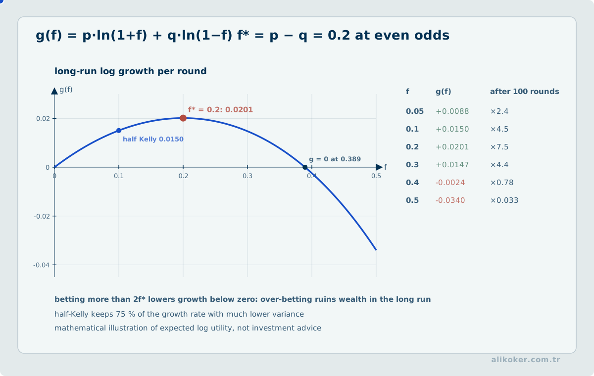
Under risk, expected value can be written as:

E[X] = Σ p(s) * x(s)

When money, safety, time, or service loss has a nonlinear value to the decision maker, expected utility is more appropriate than raw expected monetary value.

A risk-averse decision maker may legitimately prefer a lower-variance alternative even when two alternatives have the same expected value. The preference is represented by the utility function rather than dismissed as irrational.

5.3. Decision Trees

Decision nodes and chance nodes should remain distinct:

[Decision]
  |-- A --> (Uncertain state) -- p1 --> outcome
  |                         -- p2 --> outcome
  |
  -- B --> (Uncertain state) -- p1 --> outcome
                            -- p2 --> outcome

Decision trees are useful for sequential choices in which information arrives over time.

5.4. Value of Information

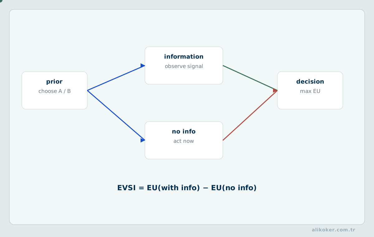
Additional sensing or analysis is valuable only if it can improve the decision enough to justify its cost. Conceptually, perfect information value is the difference between:

expected best outcome with perfect information
-
expected best outcome with current information

More data is not automatically more valuable data.

Calculating the economic value of information. Suppose two alternatives A and B face high demand with probability 0.4 and low demand with probability 0.6. Their net outcomes in the high/low states are A: (100, −20) and B: (60, 40) units. Without further information, expected outcomes are E[A] = 0.4·100 + 0.6·(−20) = 28 and E[B] = 0.4·60 + 0.6·40 = 48, so B is preferred. With perfect information before the decision, select A under high demand and B under low demand, yielding 0.4·100 + 0.6·40 = 64. Expected value of perfect information is EVPI = 64 − 48 = 16 units. Under the same payoff definition, this is a theoretical upper bound on what perfect information is worth. An imperfect test must be evaluated separately using its sensitivity, false-alarm rate, and acquisition cost.

Unit 6: Multi-Criteria Decision Making

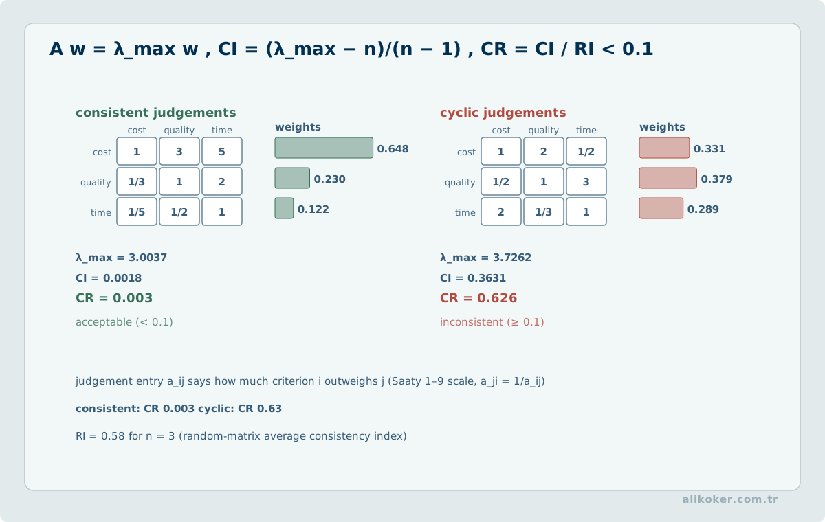
Operational decisions commonly involve cost, quality, time, risk, resilience, and sustainability at the same time.

6.1. Weighted Scoring

A simple form is:

score(a) = Σ w_j * r_aj

where w_j is a criterion weight and r_aj is the normalized performance of alternative a.

Two conditions dominate the result:

1. criterion values must be normalized consistently;
2. weights must represent real preferences.

Making weights sum to one is mathematically convenient; it does not make questionable weights correct.

6.2. TOPSIS

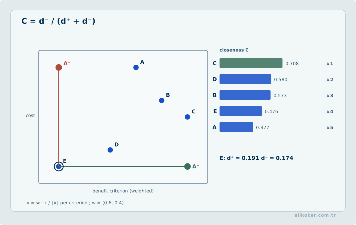
TOPSIS ranks alternatives by proximity to an ideal solution and distance from a negative ideal. A typical workflow is:

decision matrix
 -> normalization
 -> criterion weights
 -> ideal / negative-ideal points
 -> distances
 -> relative closeness
 -> ranking

Sensitivity to weights and normalization should be examined before treating the ranking as stable.

6.3. Pareto Reasoning

An alternative can be Pareto-efficient when improving one objective necessarily worsens another. Multi-objective problems naturally produce a set of efficient trade-offs rather than a single universal optimum.

A DSS should help the decision maker understand this frontier instead of silently collapsing every preference into one opaque score.

Unit 7: Multi-Objective Optimization and Model-Driven DSS

7.1. Linear and mixed-integer Optimization

Linear programming has a linear objective and linear constraints:

min / max  c'x
subject to Ax <= b
           x >= 0

When some decisions are discrete, mixed-integer formulations are required. Scheduling, allocation, routing, and capacity planning often contain such discrete structure.

7.2. Weighted-sum Objectives

Several objectives may be combined:

min w1*f1(x) + w2*f2(x) + wk*fk(x)

The weights are part of decision policy; they should not be hidden as purely technical tuning parameters.

7.3. Goal Programming

Goal programming penalizes positive and negative deviations from target values. It is useful when the decision language is closer to "stay within budget and approach the service target" than to a single abstract objective.

7.4. Epsilon-constraint Method

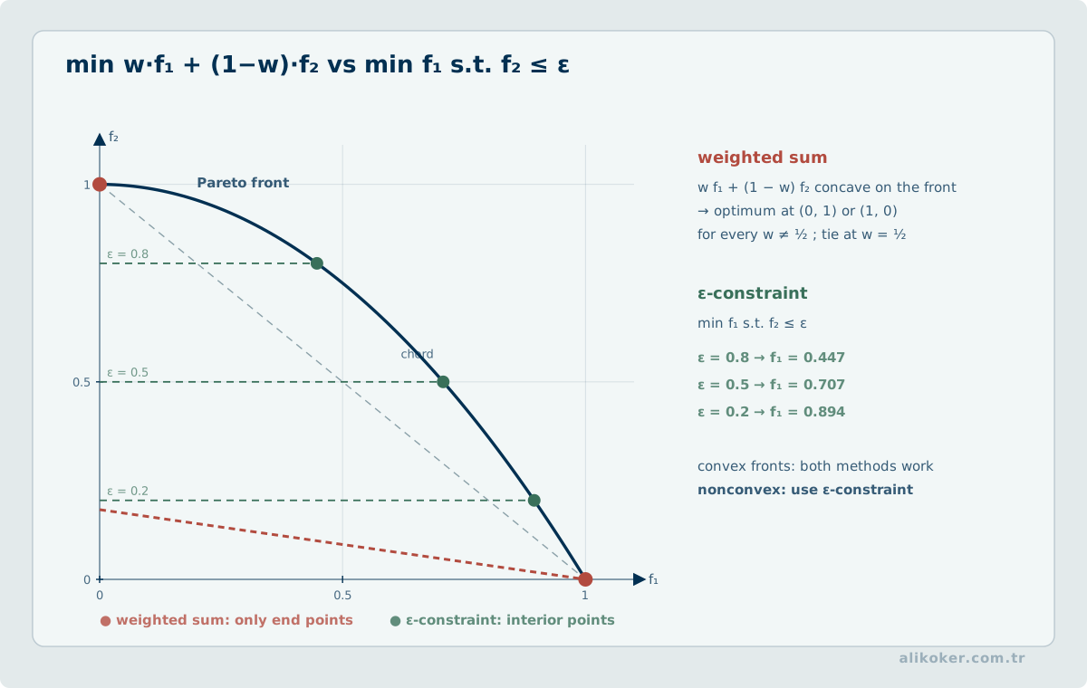
One objective is optimized while others become explicit bounds:

min cost
subject to service_level >= ε1
           risk <= ε2

This can directly encode policies such as "never fall below this service level."

7.5. Verifying Solver Output

An "optimal" solver status does not prove that the real decision problem has been solved correctly. Verification should examine:

• units and signs,
• boundary conditions,
• constraint tolerances,
• integrality,
• unexpectedly inactive constraints,
• sensitivity,
• alternate optima,
• alignment with real operational constraints.

Genetic Algorithms and Their Applications provides a complementary view of heuristic optimization.

7.6. Convexity and the Geometry of the Feasible Region

An optimization problem is shaped not only by the name of its objective but by its geometry. In a convex set, the line segment between two feasible points remains feasible. For a convex objective,

f(lambda x + (1-lambda)y)
<= lambda f(x) + (1-lambda) f(y)

for 0 <= lambda <= 1.

In convex minimization, every local minimum is also global. This separates merely finding a stationary point from having a mathematical guarantee about global optimality.

For a DSS, convexity is not an abstract convenience. It affects solution guarantees, solver scalability, and the reliability of sensitivity interpretation.

7.7. Linear Programming, Simplex, and interior-point Methods

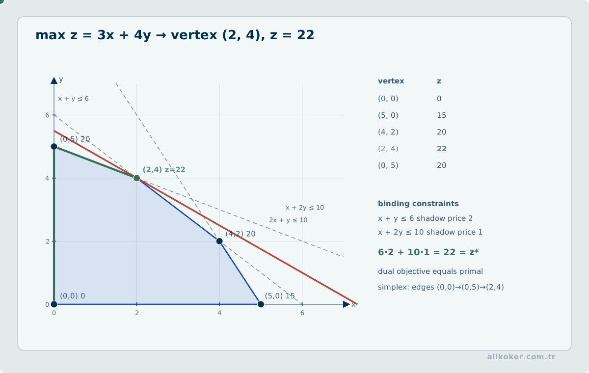
In linear programming the objective and constraints are linear, so the feasible region is a polyhedron. Under suitable conditions, at least one optimum occurs at a vertex.

The Simplex method can be viewed as moving among adjacent basic feasible solutions. Interior-point methods instead approach optimality through the interior rather than following a sequence of vertices.

Which approach is preferable depends on problem size, sparsity, numerical structure, warm-start requirements, and solver implementation. A DSS should record the model structure and solver contract rather than merely the algorithm name.

7.8. Duality and Shadow Prices

Dual variables can be associated with constraints of a primal optimization problem. In linear programming, suitable conditions produce equality between primal and dual optimal objective values. This relationship supports both optimality checks and interpretation of constrained resources.

The local effect of relaxing a right-hand-side constraint can be interpreted through a shadow price. It is not a universal fixed price: when the active set or basis changes, the local sensitivity can also change.

Dual information therefore helps answer not only "what is the solution?" but also "which scarce resource is limiting the decision?"

A shadow price describes the local change in an optimal objective value when the right-hand side of a resource constraint is perturbed. It remains valid only while the relevant active-set structure persists. If production x is maximized subject to x≤8 and x≤10, increasing the first bound from 8 to 9 raises the optimum by one; beyond 10, further increases have no value. Extrapolating the original dual coefficient across every capacity increment would therefore be misleading. A decision-support result should report the range over which a marginal value is meaningful.

7.9. Lagrange Multipliers and KKT Conditions

For an equality-constrained problem, the Lagrangian can be written as

L(x,lambda) = f(x) + lambda^T h(x).

With inequalities, the Karush-Kuhn-Tucker framework combines

primal feasibility
dual feasibility
stationarity
complementary slackness.

Under convexity and suitable regularity conditions, KKT conditions strongly characterize optimality. In a nonconvex problem, a KKT point is not a guarantee of global optimality.

Within a DSS, KKT theory is useful for interpreting solver status and dual information rather than for reimplementing a solver by hand.

Complementary slackness in the KKT conditions identifies when an inequality constraint is active at the optimum. Minimizing f(x)=(x−3)² subject to x≤2 gives x=2. With g(x)=x−2≤0, stationarity yields 2(x−3)+λ=0, so λ=2 for the active bound. Replacing the bound by x≤4 makes it inactive: the optimum is x=3 with λ=0. In this one-dimensional convex example the conditions are sufficient. For a general nonlinear nonconvex problem, solving the KKT equations alone does not certify a global optimum.

7.10. First- and second-order Optimization Methods

Gradient descent uses first-order information. A step size that is too large can oscillate or diverge, while an excessively small one wastes iterations.

Newton's method uses a local quadratic model through the Hessian:

H(x_k) p_k = -grad f(x_k)
x_(k+1) = x_k + p_k.

When a full Hessian is too expensive, quasi-Newton methods such as BFGS iteratively approximate curvature. For nonsmooth objectives, subgradient methods may apply; for composite objectives g(x)+h(x) with a simple proximal term, proximal-gradient methods can exploit structure.

Methods should not be compared only by iteration count. Linear-algebra cost per iteration, memory use, parallelism, constraint handling, and target tolerance all matter.

7.11. Network Flow as an Optimization Structure

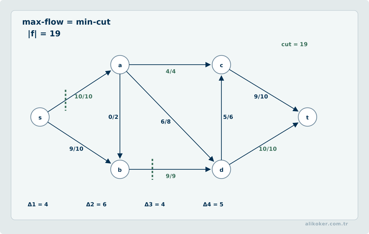
Networks with capacities, costs, and flow conservation create natural optimization models. Maximum flow, minimum-cost flow, and assignment can be expressed as generic linear or integer programs, yet specialized graph algorithms often exploit structure more efficiently.

This is an important modeling lesson: structure need not be destroyed merely to fit a general solver. Specialized algorithms and general optimization models should be compared in terms of correctness, flexibility, maintainability, and performance.

7.12. Feasible, Infeasible, Unbounded, and Optimality Gap

A solver terminating does not imply that an optimum has been found. The basic states should be distinguished:

• feasible: at least one solution satisfies every constraint;
• infeasible: the constraints cannot be satisfied together;
• unbounded: the objective can improve without bound inside the feasible region;
• optimal: no better feasible solution exists within the declared tolerance;
• time/iteration limit: resource limits were reached before mathematical search was completed.

For mixed-integer problems, the optimality gap summarizes the separation between the best feasible incumbent and a mathematical bound. A decision record should preserve not only decision variables but also solver status, gap, tolerances, model version, and data snapshot.

Unit 8: Simulation-Based Decision Support

Optimization typically asks which action is best; simulation often asks how a proposed policy behaves.

8.1. Monte Carlo Simulation

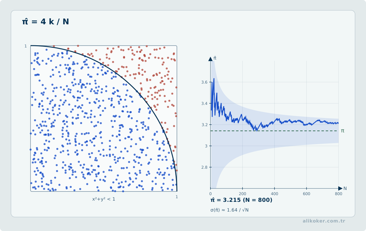
Random inputs are repeatedly sampled to estimate an outcome distribution:

for each trial:
    demand  ~ distribution
    duration ~ distribution
    failure ~ distribution
    compute outcome
summarize outcome distribution

Percentiles, tail losses, and threshold exceedance probabilities can be more informative than a single mean.

8.2. Discrete-event Simulation

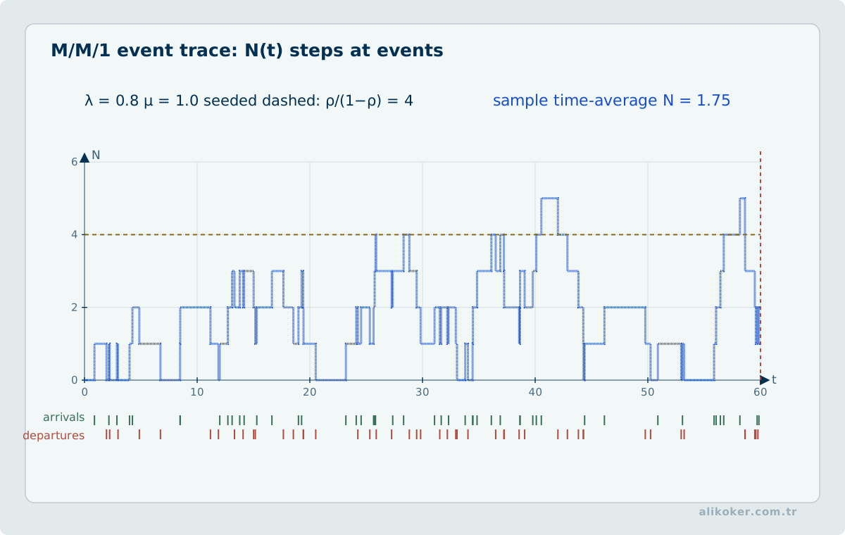
In queues, maintenance, logistics, and shared-resource systems, state changes when events occur. Discrete-event simulation is well suited to waiting times, utilization, bottlenecks, and congestion.

8.3. Optimization Plus Simulation

The two techniques can be composed:

optimization -> candidate policy
                    |
                    v
                simulation
                    |
            robustness / risk
                    |
                    v
              policy choice

This filters nominally attractive solutions that are fragile under realistic variability.

8.4. Scenario Pairing and Simulation Budgets

Comparing two decision policies under the same randomly generated demand, failure or service-time conditions can reduce the noise in the estimated difference. The common random numbers technique uses paired scenarios rather than independently generated scenarios for every policy. For a loss difference D_i = L_A(ω_i) − L_B(ω_i), the evidence consists of D̄ and its sampling uncertainty; comparing two apparently different standalone means is insufficient. Pairing can lower variance when outcomes are positively correlated across policies, but this benefit is not automatic.

Reusing a seed makes a simulation repeatable; independent replications with different seeds test whether the conclusion depends on a single realization. Alongside average loss, report tail quantiles, exceedance probabilities and thresholds relevant to the decision. Standard Monte Carlo can be inefficient for rare but consequential events. If importance sampling is introduced, the stability of its weights and coverage of the proposal distribution require separate checks.

Unit 9: Representing Uncertainty

Uncertainty is not one mathematical object.

9.1. Probabilistic Uncertainty

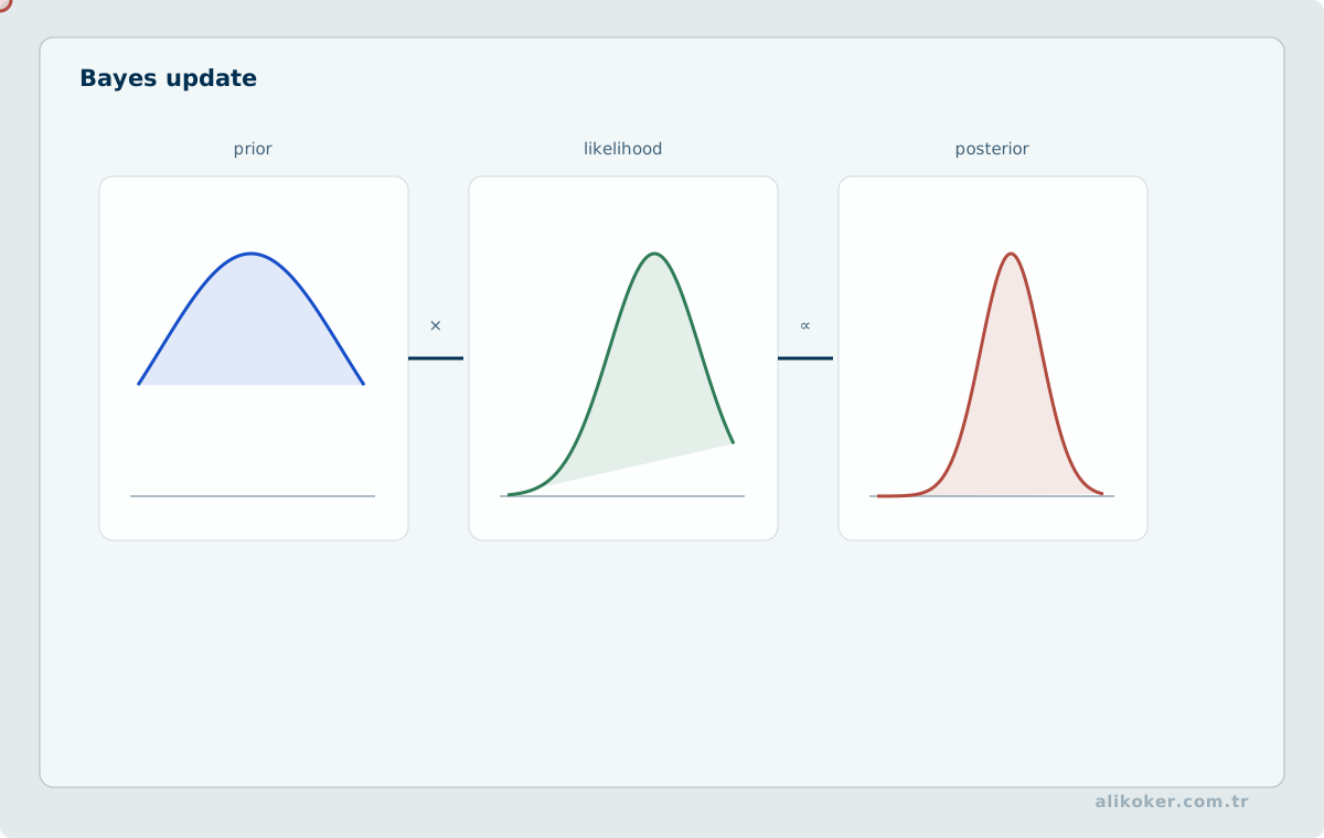
Probability distributions are appropriate when frequencies or credible probabilistic models are available. Parameter uncertainty should be separated from irreducible stochastic variation where possible.

9.2. Fuzzy Uncertainty

Concepts such as "high risk" or "acceptable temperature" may have gradual boundaries. Fuzzy membership represents degree of membership, not event probability.

9.3. Model Uncertainty

The model structure itself may be uncertain. If plausible models disagree, a narrow parameter confidence interval can understate the real uncertainty. Scenario sets or model ensembles may be more appropriate.

9.4. Robust and Cautious Decisions

Robust optimization seeks solutions that perform acceptably across a defined uncertainty set. Caution does not always mean selecting the mathematically worst case; reversibility, monitoring, and the ability to adapt after new information arrives also matter.

9.5. Sequential Decisions: MDPs and POMDPs

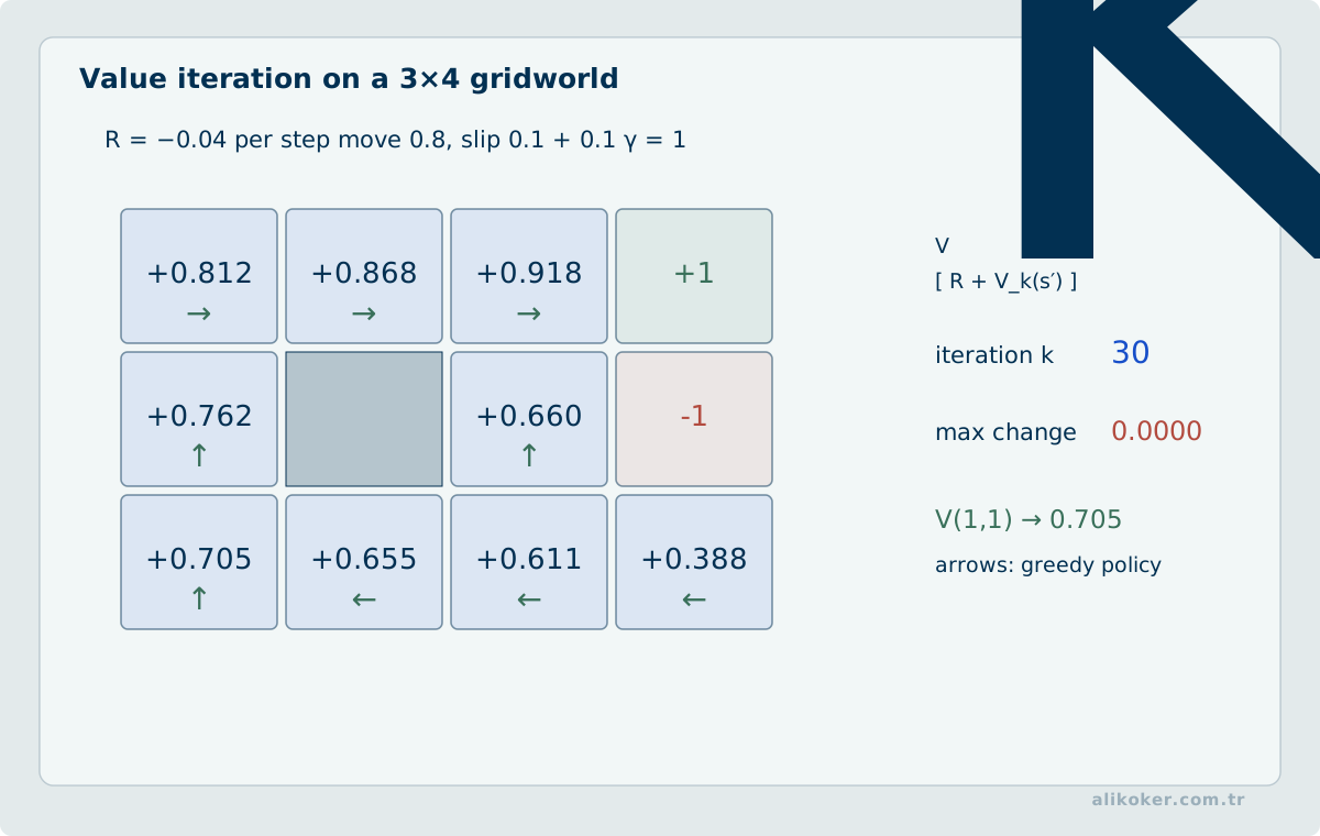
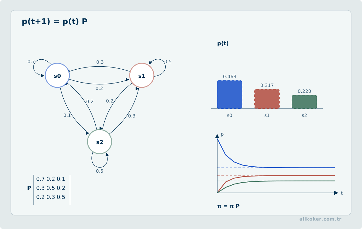
Markov decision processes combine state, action, transition probability, and reward. When the true state is only partially observed, a POMDP reasons over a belief state.

These formulations differ from one-shot ranking because they seek a policy for acting over time.

9.6. Types of Uncertainty and Decision Displays

A point forecast can conceal measurement and sampling uncertainty from its reader. Yet labeling different kinds of intervals simply as “confidence intervals” is also misleading. A confidence interval for a parameter, a prediction interval for a future observation and a posterior credible interval answer different questions. An uncertainty display should identify the quantity covered, the assumptions used and the subset of data on which the assessment rests.

Comparable quantiles or quantile dotplots for multiple choices can expose skewness hidden by a conventional error bar. Visual detail must not displace the decision variable's meaning: thresholds and color scales should not turn continuous uncertainty into sharply defined categories unsupported by the distribution. Overlapping intervals do not automatically establish equal decisions, nor does a lack of overlap by itself establish a meaningful decision difference; the difference in decision loss must be evaluated directly.

Unit 10: Data-Driven DSS, Prediction, and Machine Learning

In a modern DSS, prediction is one layer in a larger decision chain.

observation -> features -> prediction
                         |
                         v
                 threshold / cost
                         |
                         v
                       action

10.1. Predictive Accuracy Is Not Decision Value

The more accurate predictive model is not guaranteed to produce better decisions. When false-positive and false-negative costs differ, the operating threshold should reflect those costs.

For rare events, a high accuracy number can be achieved by an unusable classifier that predicts the majority class everywhere. Metrics such as precision-recall behavior, calibration, cost matrices, and downstream decision utility should be considered together.

Statistical Learning and Machine Learning develops the predictive modeling foundation in more detail.

10.2. Calibration

If events assigned an 80% probability occur roughly 80% of the time over an appropriate population, the model is well calibrated in that sense. Calibration can matter more than ranking quality when probabilities feed directly into expected-cost calculations.

10.3. Distribution Shift

When production data moves away from the training distribution, the decision behavior may change. A DSS should monitor not only model metrics but also:

• input distributions,
• missingness,
• class prevalence,
• calibration,
• threshold behavior,
• post-decision outcomes.

10.4. Turning Predicted Fault Probability into a Maintenance Decision

A model's predicted fault probability p is not itself a maintenance action. Suppose preventive intervention costs 400 units, while doing nothing incurs an additional loss of 2000 units if the machine fails and zero if it remains healthy. Under this simplified one-period decision, expected intervention cost is 400 and expected waiting cost is 2000p. Preventive maintenance has lower expected cost when p > 0.20. This threshold depends on both probability calibration and cost assumptions; it is not universal across assets.

The calculation assumes perfect intervention, fixed costs, and no intermediate alternatives. In practice, intervention success rate, spare-part lead time, production constraints, and potential harm to people change the decision model. If probability calibration is poor, interpreting a model score of 0.30 as a real thirty-percent event frequency may cause costly errors. A responsible decision-support system therefore separates prediction, economic consequences, authority to act, and measurement of actual outcomes.

Unit 11: Intelligent DSS and Decision Intelligence

11.1. From Expert Systems to Intelligent Support

Rule-based systems encode domain logic as conditions and conclusions. Their strengths include explicit rules and repeatability in narrow domains; their weaknesses include knowledge-acquisition cost, rule conflicts, and maintenance.

Modern intelligent DSS architectures can combine rules, machine learning, optimization, search, and agents. Artificial Intelligence provides the broader theoretical context.

11.2. Assistance, Support, Augmentation, and Automation

Human-machine allocation can be viewed at several levels:

• decision assistance: retrieve information or perform calculations,
• decision support: expose alternatives and consequences,
• decision augmentation: combine complementary human and machine strengths,
• decision automation: select and execute actions within defined authority.

As automation increases, validation, authorization, rollback, and operating boundaries become more important.

11.3. Decision Intelligence

Decision intelligence is a contemporary framing that focuses on how decisions are defined, executed, monitored, and improved, rather than treating AI or data science as prediction-only disciplines. It is not one international standard or a single algorithm family; it is used as an integrative approach connecting organizational decision processes with analytics and AI.

Unit 12: Human Factors, Explanations, and Group Decisions

12.1. Bounded Rationality

Real decision makers have limited time, attention, and computational capacity. The role of a DSS is not to maximize dashboard density but to make the decision-relevant distinctions visible.

12.2. Automation Bias

A consistent-looking system recommendation can receive more trust than its evidence warrants. Interfaces can reduce this risk by exposing:

• missing data,
• model validity limits,
• uncertainty,
• critical assumptions,
• contradictory evidence,
• alternatives.

12.3. Explanation Is Not Correctness

An articulate explanation does not prove that a recommendation is correct. An explanation should state which question it answers:

• Which inputs mattered?
• Which rule fired?
• Which constraint limited the solution?
• Why was an alternative rejected?
• Which change would reverse the decision?

12.4. Feature Attribution, Counterfactual Explanations, and Causality

A feature-attribution explanation distributes a model output among inputs under a specified model and reference distribution; it does not establish causal effects. With correlated features, assigned contributions may depend on the attribution method and background sample. Global importance rankings and local explanations for one decision are different objects.

A counterfactual explanation asks which input changes would alter a model prediction. Mutable and immutable features, physical constraints, and jointly varying variables must be specified; otherwise a counterfactual example may not represent an actionable intervention. Causal claims additionally require intervention assumptions, consideration of confounders, and explicit limits on observational evidence.

Association in observational data does not establish how an outcome would change under intervention. A causal directed acyclic graph (DAG) can make assumed pathways and confounding explicit, but the graph is not automatically identified from data. Back-door adjustment requires selecting variables that block relevant confounding paths without opening spurious ones.

A propensity score summarizes treatment probability conditional on observed covariates. Covariate balance, positivity, and the absence of unmeasured confounding remain necessary for the intended interpretation. Instrumental-variable methods require different assumptions, including instrument relevance and an exclusion restriction. High predictive accuracy does not establish these identification conditions.

12.5. Group Decisions

Group DSSs are not merely electronic voting systems. Stakeholders may differ in:

• objectives,
• authority,
• access to information,
• risk tolerance,
• objection and approval rights.

A useful decision record can retain rationale and dissent rather than only the final selection.

Cognitive Systems Engineering provides a deeper treatment of human factors and situation awareness.

Unit 13: Generative AI and RAG Inside Decision Support

Large language models can be valuable for natural-language interaction, document analysis, explanation, and hypothesis generation from unstructured information. Their output is not, by itself, authoritative decision evidence.

13.1. Separation of Roles

user question
   |
   v
LLM: interpret intent and information need
   |
   +--> validated data query
   +--> document retrieval / RAG
   +--> deterministic calculation tool
   +--> optimization / simulation
   |
   v
evidence + result + uncertainty
   |
   v
LLM: produce an understandable presentation
   |
   v
human approval / authorized action

The LLM routes work to verifiable tools instead of imitating reliable computation. Retrieval-Augmented Generation (RAG) covers grounded generation in more detail.

13.2. Principal Risks

• hallucination,
• stale or incorrect context,
• fabricated attribution,
• prompt injection and authority boundary violations,
• using text generation for structured arithmetic,
• assigning nondeterministic generation to decisions that require deterministic execution.

For high-impact settings, generative models are better positioned as retrieval and explanation layers around validated decision services than as unconstrained decision authorities.

Unit 14: DSS Software Engineering and Lifecycle

The gap between a DSS prototype and a production DSS is often defined by engineering controls rather than by the core algorithm.

14.1. Spreadsheet Prototypes

Spreadsheets remain effective for making small models visible, exploring what-if questions, conducting sensitivity analysis, and working interactively with domain experts. Their limits become significant in multi-user, high-volume, or critical production use:

• hidden cell dependencies,
• version divergence,
• concurrent editing,
• access control,
• automated testing,
• data-source integrity.

Production migration should turn formulas and assumptions into explicit model contracts, service boundaries, and testable components.

14.2. Versioning

These elements should be versioned together when they jointly determine a decision:

data schema
+ data transformation
+ feature definition
+ model
+ optimization parameters
+ business rules
+ decision threshold
+ decision explanation

Versioning only the model artifact is not enough for reproducibility.

14.3. Verification and Validation

• Verification: did we implement the specified model correctly?
• Validation: is the model sufficiently appropriate for the real decision problem?

Correct solver implementation is verification; checking whether the objective reflects real operational value is validation.

Software Engineering provides the broader lifecycle context.

Unit 15: Performance, Reliability, and Operational Design

A recommendation can lose all value if it arrives after the decision window closes. Algorithmic quality and temporal behavior are both requirements.

15.1. Latency, Throughput, and Freshness

Three notions must remain separate:

• computation latency,
• end-to-end decision latency,
• age of the data used.

A model may respond in 20 ms while using data that is 24 hours old. That is fast computation, not necessarily real-time decision support.

15.2. Controlled Degradation

Fallback behavior should be designed before failures occur:

normal decision support
 -> advanced model unavailable
 -> validated baseline rule / last trusted model
 -> explicit degraded state
 -> human approval

Silently switching to stale data or a different model makes the decision trail ambiguous.

15.3. Caching

Expensive results may be cached, but a correct cache key may need data version and model version in addition to user inputs. Otherwise the system can return an incorrect answer very efficiently.

Unit 16: Measuring Decision Quality

16.1. Model Metrics and Decision Metrics

DSS evaluation can be separated into four levels:

1. Data quality: completeness, accuracy, freshness, representativeness.
2. Model quality: predictive performance, calibration, optimization validity, robustness.
3. Decision-process quality: decision time, user workload, explainability, override behavior.
4. Outcome quality: cost, service, safety, loss, objective attainment.

A model metric can improve while the real outcome worsens. Controlled rollout should therefore measure downstream effects.

Better predictive accuracy is not a guarantee of better decisions. Reducing mean absolute error for maintenance risk estimates is useful, but when only two maintenance slots are available, the operational task is to select the two interventions expected to prevent the greatest loss. A decision metric must account for intervention cost and the impact of failure. The same applies to reporting: displaying a number without its denominator, observation period, missing-data rate and uncertainty may imply false precision. Decision quality must ultimately be examined through reproducible calculation and feedback on decisions taken.

16.2. Counterfactual Evaluation

Production systems normally observe the outcome of the selected action but not what would have happened under the unselected alternatives. Evaluating decision policies is therefore harder than evaluating a static predictor.

Where randomization is infeasible, historical controls, matching, causal models, or simulation may help, but each introduces assumptions that should be documented.

For observational decision logs, the outcome of an unchosen action is not observed directly. Random assignment can identify intervention effects under suitable experimental conditions; blocking and stratification control known sources of variability during design. Without experiments, off-policy evaluation methods such as importance weighting require correctly specified action probabilities and sufficient overlap.

Selection bias and measurement error can distort estimated decision value independently of predictive model scores. Policy comparisons should consider uncertainty, costs, constraints, and outcome variation rather than mean reward alone.

16.3. Human Override

A rejected recommendation is not automatically a user error. Override patterns may reveal:

• contexts where the model is weak,
• information missing from the system,
• inadequate explanations,
• excessive false alarms.

Override behavior is a diagnostic signal rather than a metric that should always be minimized.

16.4. Robustness and Temporal Context in Decision Analytics

Robust statistics asks how much an estimator degrades under small departures from an idealized model. When decision-support outputs are derived from many scenarios or simulation runs, the median and MAD reduce the leverage of exceptional runs; influence functions and breakdown points provide a more formal description of how strongly a decision metric can be shifted by extreme observations. In heavy-tailed or contaminated data, decisions based only on the mean and standard deviation can be misleading.

• Measure how much one extreme observation changes the decision score through sensitivity analysis.
• Test whether rankings remain stable when the time window changes.
• Separate model score from decision threshold and use human review in uncertain regions.

16.5. Prediction Performance Is Not Decision Utility

A predictive model is not itself the outcome of a decision-support system. If event probability is p, a false action costs C_FP, and a missed event costs C_FN, then the expected loss of acting is (1-p)C_FP, while the loss of not acting is p C_FN. Acting has lower expected loss when p > C_FP/(C_FP+C_FN), subject to calibrated probabilities and correctly specified costs.

Models with similar ROC-AUC can have very different operational value when calibration differs. Intervention capacity, human approval, sensitivity to costs, and reversal expenses must be monitored independently of headline model scores.

16.6. Explanation Stability and Counterfactual Feasibility

If an explanation changes completely under small, irrelevant input perturbations, its reliability as an operational justification is questionable. Stability can be assessed through changes in feature rankings, consistency of attribution signs, and sensitivity to the reference distribution. Fidelity to the underlying model differs from the accuracy of a decision: the explanation should represent relationships actually used by the model.

A counterfactual recommendation is not selected solely by minimum numerical distance. Change cost, physical feasibility, authority to act, and possible side effects must be considered. Evaluation should report predictive accuracy, explanation stability, fidelity, and human decision error as distinct outcomes.

Unit 17: Governance, Risk, and Responsible AI

As decision impact grows, model management becomes part of organizational risk management.

NIST AI Risk Management Framework 1.0 provides a voluntary, sector-agnostic structure for managing AI risks across the lifecycle. NIST's 2024 Generative AI Profile specializes that framework for generative-AI risks. ISO/IEC 23894:2023 provides AI risk-management guidance, while ISO/IEC 42001:2023 specifies an organizational AI management system. ISO/IEC 25010:2023 defines the current product quality model for software and ICT products.

These standards do not replace the decision model. Their value is in structuring questions of responsibility, lifecycle control, measurement, and governance.

17.1. Minimum Control Areas for high-impact Decisions

• data and model lineage,
• access control and authorization,
• data minimization,
• threat modeling,
• independent testing,
• representation and bias analysis,
• human approval and override,
• action boundaries,
• rollback,
• incident records,
• periodic reassessment.

Decision risk is not limited to systems labeled as AI. A wrong optimization target, corrupted data, or a misleading interface can create severe decision risk without machine learning.

Unit 18: End-to-End Example — Maintenance and Capacity Planning DSS

Consider a system that schedules maintenance across many assets while preserving service capacity.

18.1. Inputs

• equipment health indicators,
• predicted failure probabilities,
• maintenance duration,
• spare-parts availability,
• workforce capacity,
• service demand,
• maintenance windows.

18.2. Decision Variables

• which asset to maintain and when,
• which team to assign,
• which reserve resource to activate.

18.3. Objectives

• reduce unexpected failure risk,
• reduce total maintenance cost,
• preserve service capacity,
• limit overtime.

18.4. Architecture

sensors / maintenance records
          |
          v
data quality + temporal alignment
          |
          +--> health prediction
          |
          +--> failure probability
          |
          v
mixed-integer optimization
          |
          v
candidate maintenance plans
          |
          +--> Monte Carlo stress test
          |
          v
risk / cost / service trade-offs
          |
          v
decision-maker interface
          |
          v
approval -> work order -> observed outcome
          |
          +--------------------> feedback

The predictive model estimates failure risk; it does not determine the maintenance plan by itself. Optimization combines capacity, cost, staffing, and timing constraints. Simulation evaluates how robust the nominal plan is under uncertainty. A human decision maker can alter the recommendation when relevant field information is absent from the model.

This is why a DSS is an end-to-end decision system rather than a synonym for an AI model.

Unit 19: Evidence-Aware Analytical Decision Support

One of the most dangerous design shortcuts in decision support is to collapse analysis into a single score and present that score as a judgment about the real world. A more defensible design produces a support profile that exposes data scope, evidence, limitations, method agreement, robustness, and the conditions under which an interpretation could change.

The key separation is:

source data
   ↓
analytical signal
   ↓
finding
   ↓
support / limitation profile
   ↓
human interpretation and decision

The analytical system may show that a pattern is repeatedly supported inside the available data. It does not, by itself, establish the real-world meaning, intent, or importance of that pattern.

19.1. Data Sufficiency Is Part of the Result

A decision-support system should report not only what it found but what data the result actually represents.

Useful questions include:

• Is the analytical scope complete or partial?
• What fraction of observations contain usable timestamps?
• Are direction, category, or duration fields incomplete?
• Is the time range sufficient for the requested comparison?
• Does more data remain outside the loaded analytical scope?

A useful scope model is:

Analysis Scope
├─ observed records
├─ loaded records
├─ observation period
├─ per-field coverage
├─ complete / partial scope
└─ evaluability conditions

Missing information is not the same as a zero-valued observation. Treating unknown direction as “no direction,” for example, creates a false negative rather than an honest statement of uncertainty.

19.2. A Finding Support Profile

Instead of inventing one confidence percentage, the system can expose several dimensions:

Finding Support Profile
├─ number of source observations
├─ number of distinct signal families
├─ agreement across methods
├─ field coverage
├─ complete / partial scope
└─ known limitations

These are not probabilities of truth. Three analytical signals supporting a pattern mean that the finding has multiple forms of support inside the current data; they do not imply that the finding is “90% true” in the real world.

19.3. Signal Diversity Is Not Metric Count

Five metrics do not necessarily provide five independent pieces of evidence.

For example:

total event count
average daily count
high-volume percentile

may all be derived from the same underlying volume information.

By contrast:

volume
persistence over time
direction balance
structural network position
period-over-period change

represent different signal families.

Decision support should therefore distinguish independent analytical dimensions from repeated transformations of the same information.

19.4. Limitations Are Not counter-evidence

A limitation narrows the interpretation:

timestamps are incomplete
the observed network is partial
too few days are evaluable
a field has low coverage

A balancing observation points in another analytical direction:

high volume
but little persistence

strong structural position
but only inside a small observed subgraph

one temporal method flags a day
but other methods do not

The statement “no counter-evidence was found” must never be rewritten as “the finding is confirmed.”

19.5. Agreement Across Methods

If multiple methods highlight the same region of a time series, that agreement can strengthen analytical support.

For example:

robust deviation
+
exponentially weighted average
+
cumulative-change method

may identify the same period.

However, methods that share the same data and similar assumptions are not independent experiments. The appropriate conclusion is that multiple analytical methods agree within the current data, not that the real-world interpretation has been proven.

19.6. Robustness

Robustness asks whether a finding survives small, reasonable analytical changes.

Examples:

• Does the finding remain when the observation period shifts?
• Does it persist when the most recent days are excluded?
• Does the first half of the data show a compatible pattern?
• Does a structural result change when the observed graph changes slightly?
• Does lower field coverage invalidate the interpretation?

Robustness is not proof of truth. It measures dependence on analytical choices.

19.7. Sensitivity

Sensitivity asks a more direct question:

What would have to change for this interpretation to change?

For a relationship finding, important variables may include the observation period, persistence across days, direction coverage, graph scope, or the boundary between comparison periods.

For a temporal finding, important variables may include the number of evaluable days, daily sample density, the baseline period, and treatment of extreme values.

This information gives the decision maker a map of assumptions rather than only a conclusion.

19.8. Local what-if Analysis

A what-if operation should not silently acquire new data.

A safer model is:

current analytical snapshot
        ↓
explicit scenario transformation
        ↓
recompute the same metrics
        ↓
compare baseline and scenario

Examples include:

• exclude the most recent seven days,
• analyze only the first half,
• exclude one category,
• use only observations with complete timing information.

The scenario transformation must be explicit so that the comparison can be reproduced.

19.9. Recommending the Next Analytical Step

A valuable DSS function is not “decide for the user” but recommend what to inspect next.

Examples:

weak temporal coverage
 -> inspect time distribution before interpreting change

strong structural signal but partial graph
 -> avoid generalizing outside the observed graph

only one anomaly method agrees
 -> compare with additional temporal methods

finding has source evidence
 -> inspect the underlying observations

This turns automation into structured analytical guidance.

19.10. Capability Boundaries

A language or analytical layer may propose an action without being authorized to execute it.

A safer architecture is:

interpretation / intent
   ↓
proposed analytical action
   ↓
capability and authorization check
   ↓
allowed tool
   ↓
result

The reasoning layer therefore cannot expand its own data-access or execution privileges.

19.11. Determinism and Reproducibility

The same:

analytical snapshot
+ selected finding
+ user request

should produce the same decision-support result.

If snapshots are versioned, a past finding can be reproduced against the same analytical state. When new data arrives, a new version is created instead of silently changing the context of an old conclusion.

19.12. Conversational Context

A user should be able to continue:

"show the strongest change"
"why?"
"what are the limitations?"
"what would change it?"
"what should I inspect next?"

without restating the whole query.

Conversation state can therefore track the previous intent, current result, selected finding, selected evidence, active period, and analytical snapshot version.

State management is itself a correctness concern: a new turn that does not produce new analytical data should not silently reset the user's current selection.

19.13. Synthetic Example

Suppose a maintenance platform analyzes 60 days of equipment events.

The analytical layer finds:

• rising event volume for one equipment group,
• persistence across the last 12 days,
• agreement between two temporal methods.

An evidence-aware DSS could present:

Finding:
  Event volume increased in the recent period.

Support:
  - 43 source events
  - volume and persistence signals
  - two temporal methods agree

Limitations:
  - event category is missing in some observations
  - non-maintenance downtime is not coded separately

Sensitivity:
  - removing the most recent seven days weakens the increase

Next step:
  - inspect the source events together with the maintenance calendar

The output communicates both the finding and the boundary of the finding.

19.14. Engineering Checklist

Ask:

1. Is the analytical scope explicit?
2. Is missing data distinguished from zero?
3. Can findings be traced to source observations?
4. Are correlated metrics being counted as independent evidence?
5. Are limitations shown next to the finding?
6. Are balancing observations considered?
7. Is method agreement described without overclaiming?
8. Is robustness distinguished from truth?
9. Are sensitivity conditions visible?
10. Is what-if analysis explicit and reproducible?
11. Does the system support analysis rather than issue real-world judgments?
12. Are proposed actions separated from execution authority?
13. Does the same snapshot and request produce the same result?
14. Can conversational state mix stale and current findings?

This model turns decision support from a score-producing automation layer into an auditable analytical reasoning aid.

19.15. Evidence Sufficiency and the Value of Information Before a Decision

An inability to decide does not always indicate a weak algorithm. Missing records, ambiguous references, or conflicting sources may simply leave the decision underdetermined. Two actions must then be compared: deciding with available information and seeking clarification. The expected value of additional information depends on the reduction in decision error cost relative to the delay and effort required to obtain it. The same threshold is inappropriate for a descriptive summary and a difficult-to-reverse record action.

Decision prerequisites should be checked independently. A query can be understood while its result set is stale; an evidence record may exist but lie outside the user's authorized scope; a numerical finding may be computed correctly yet described with the wrong coverage. In such cases the system should identify the missing prerequisite rather than choose the nearest-scoring alternative. This keeps classification accuracy separate from execution safety.

A useful explanation is not a dump of every intermediate model score. It presents the data interval, criteria, excluded sources, and uncertainties that could materially change the result. A compact and verifiable justification is preferable to a lengthy account whose evidence cannot be traced.

Unit 20: Verified Structured Response Generation

A decision-support system can compute the right result and still communicate it incorrectly. Free-form language adds a new failure surface when findings contain numbers, identifiers, directionality, scope conditions, or negation.

A safer architecture inserts a structured response pipeline between analytics and final text:

analytical result
   ↓
atomic facts
   ↓
discourse plan
   ↓
deterministic rendering
   ↓
integrity validation
   ↓
user response

20.1. Atomic Facts

The result can first be decomposed into small verifiable facts:

SUMMARY
RESULT_ITEM
COVERAGE
LIMITATION
EVIDENCE
NEXT_STEP

This representation defines what must survive before any sentence is generated: establish the data-and-fact contract before producing language.

20.2. Presentation Preferences Must Not Change Computation

A user may request a brief, detailed, plain, or technical response. These choices should alter presentation rather than analytical computation.

A rendering layer can use:

verbosity = brief | normal | detailed
register  = plain | technical

to decide which facts are shown and in what order.

20.3. Deterministic Rendering

In high-assurance decision support, the same fact set and presentation preference can produce the same textual structure.

This improves regression testing, reproducibility, and detection of number or identifier drift.

Deterministic response generation is a risk-control option rather than a universal requirement: as the consequence of a communication error rises, the design can trade linguistic freedom for stronger verification.

20.4. Response Integrity Validation

Generated text can be checked against its structured facts.

Important invariants include:

numbers
identifiers
entities
direction
evidence count
polarity
scope qualifier

If the analytical result contains 18 observations but the rendered text says 17, the defect is in presentation rather than analytics.

Likewise, “direction is unknown” must not become “communication is bidirectional.”

If validation fails, a simpler direct renderer is safer than attempting repair through new guesses.

20.5. Decision Envelope

A temporary decision envelope can preserve verifiable artifacts from one interaction:

input summary
interpreted request
selected analytical operation
parameter provenance
analysis version
structured result
evidence references
response-validation result

Its purpose is not to expose hidden reasoning. It provides an engineering-level account of observable steps.

20.6. Parameter Provenance

For critical parameters, origin matters as much as value.

period = 14 days
source = USER_LITERAL

or:

selectedFinding = 2
source = CURRENT_RESULT_SELECTION

can prevent similarity scores or guesses from silently becoming authoritative identifiers.

20.7. Premise Validation

If the user requests evidence for a second finding but the current result contains only one, the system must not invent the missing item.

Useful checks include whether the requested ordinal exists, the selection belongs to the current analysis version, the evidence reference exists, and the requested period is compatible with the result.

20.8. Safe Uncertainty

Verified NLG should treat non-answer as a valid outcome.

When data is insufficient, context is ambiguous, an item does not exist, or evidence cannot be resolved, the system should clarify or state the limitation instead of forcing the closest answer.

20.9. Separate Computation, Presentation, and Action

A robust architecture distinguishes computation, presentation, and authorized action. Success in one layer does not grant authority to another.

Verified structured response generation aims to preserve analytical truth, scope, polarity, and evidence linkage from computation to communication.

An auditable analytical recommendation needs four explicit boundaries: which observations supported it, which assumptions it requires, which alternatives were rejected and which future evidence would trigger reconsideration. Comparing failures across branches by raw count is misleading when operating hours differ; an exposure denominator such as failures / total operating hours may be necessary. Small groups are also unstable because one extra event can substantially change a rate. A technical decision report is more than a results table: it preserves definitions, data coverage, comparability and conditions under which its interpretation remains defensible.

20.10. Decision Envelopes and Inference Limits Under Partial Observation

A decision-support result needs an evidence envelope between computation and recommended action. It records the observed time range, missing-data fraction when known, model, constraints, alternatives and conditions under which a recommendation applies. Unknown missingness should be reported as unknown rather than assumed zero. A confidence score cannot be derived from source count alone and must not be presented as a calibrated probability without validation.

In a synthetic production example, two capacity plans yield equal mean output, but one has worse tail waiting time. Mean, p95, unmet demand and resource cost remain separate comparison criteria. If a weighted score is necessary, its weights and sensitivity analysis must be explicit; small changes in decision thresholds should be examined for reversals of the preferred option.

An action is not a natural consequence of a calculation. A decision-support explanation or recommendation must not change persistent data without independent authorization or operator approval.

20.11. Result Provenance and Reproducible Decisions

The same numeric metric calculated under different filters, data versions or time windows does not represent the same evidence. Results need provenance linking them to the observation set and model version used. Capturing threshold, weighting and exclusion-rule versions supports independent verification.

Reproducibility does not require copying all raw records into the decision interface. A secure reference to underlying evidence, with authorization rechecked when the reference is followed, may be sufficient. Any new action based on an older result must be revalidated against current data and permissions.

Common Design Failures

• Treating a reporting dashboard as a DSS.
• Converting a prediction score directly into an action.
• Hiding data freshness.
• Confusing probability with fuzzy membership.
• Hiding preference weights as technical constants.
• Assuming the optimization objective is identical to the real organizational objective.
• Reducing model uncertainty to one narrow confidence interval.
• Treating every human override as an error.
• Treating explanation as evidence of correctness.
• Using an LLM as a deterministic calculator or unrestricted decision authority.
• Versioning models, data, and thresholds independently.
• Leaving fallback behavior unspecified.
• Measuring success only through model metrics.

20.12. Alert Review Capacity and Decision Thresholds

An anomaly-driven decision requires more than a raw score: estimated event likelihood, intervention loss and analyst capacity matter. False positives consume review resources while false negatives leave risks unaddressed. One may minimise expected loss or maximise confirmed detections under a fixed review budget, with explicit constraints. Uncalibrated anomaly scores must not be presented as event probabilities. The red-flag and alert pipeline is developed in Anomaly Detection.

Related Courses

Decision support is inherently multidisciplinary. Probability and Statistics covers uncertainty and sampling; Statistical Learning and Machine Learning develops predictive models; Artificial Intelligence covers AI foundations; Fuzzy Logic addresses linguistic uncertainty; Genetic Algorithms and Their Applications covers heuristic optimization; Cognitive Systems Engineering addresses joint human-machine decision work; Engineering Management and Project Management provides the managerial setting; and Software Engineering provides lifecycle and quality foundations.

References

• Bubnicki, Zdzislaw. Analysis and Decision Making in Uncertain Systems. Springer, 2004. ISBN 1-85233-772-9.

• Göran Kauermann; Helmut Küchenhoff; Christian Heumann. Statistical Foundations, Reasoning and Inference: For Science and Data Science. Springer, 2021. https://doi.org/10.1007/978-3-030-69827-0
• Gupta, Jatinder N. D.; Forgionne, Guisseppi A.; Mora, Manuel (eds.). Intelligent Decision-making Support Systems: Foundations, Applications and Challenges. Springer, 2006. ISBN 978-1-84628-228-7.

• ISO. ISO 31000:2018 Risk management — Guidelines. International Organization for Standardization, 2018.

• ISO/IEC. ISO/IEC 23894:2023 Information technology — Artificial intelligence — Guidance on risk management. International Organization for Standardization / International Electrotechnical Commission, 2023.

• ISO/IEC. ISO/IEC 25010:2023 Systems and software engineering — Systems and software Quality Requirements and Evaluation (SQuaRE) — Product quality model. 2023.

• ISO/IEC. ISO/IEC 42001:2023 Information technology — Artificial intelligence — Management system. 2023.

• Mor Harchol-Balter. Performance Modeling and Design of Computer Systems: Queueing Theory in Action. Cambridge University Press, 2013.

• NIST. Artificial Intelligence Risk Management Framework (AI RMF 1.0). NIST AI 100-1, 2023. DOI: https://doi.org/10.6028/NIST.AI.100-1

• NIST. Artificial Intelligence Risk Management Framework: Generative Artificial Intelligence Profile. NIST AI 600-1, 2024. DOI: https://doi.org/10.6028/NIST.AI.600-1

• O'Callaghan, Miriam. Decision Intelligence: Human–Machine Integration for Decision-Making. CRC Press, 2023. DOI: https://doi.org/10.1201/b23322

• Peter J. Huber; Elvezio M. Ronchetti. Robust Statistics. 2nd ed. Wiley, 2009.

• Walter W. Piegorsch, Richard A. Levine, Hao Helen Zhang, Thomas C. M. Lee (eds.). Computational Statistics in Data Science. Wiley, 2022. ISBN 9781119561071.
• Naveenkumar, P.; Sharma, V.; Devarajan, G.; Abdullah, A.; Elngar, A. A. (eds.). Handbook of AI-Based Mechatronics Systems and Smart Solutions in Industrial Automation. CRC Press, 2026. DOI: https://doi.org/10.1201/9781032615790.
• Cybellium Ltd. Mastering Neural Networks. Cybellium, undated electronic edition (supplied copy).
• Zahra Zohrevand; Uwe Glässer. Should I Raise The Red Flag? A Comprehensive Survey of Anomaly Scoring Methods toward Mitigating False Alarms. arXiv, 2019. https://arxiv.org/abs/1904.06646