Genetic Algorithms and Their Applications

Genetic algorithms are population-based stochastic optimization methods inspired by evolutionary selection. Their practical value does not come from reproducing biology literally, but from maintaining a set of candidate solutions, evaluating them with an objective function, and repeatedly applying selection and variation operators.

Unit 1: Optimization and Evolutionary Computation

1.1. Optimization Problem

An optimization problem searches for parameter values that minimize or maximize an objective:

f(P1, P2, ..., PN)

The objective may be an analytical function, a simulation, an experiment, or a measurement process. Depending on context it may be called an objective, cost, loss, or fitness function.

Optimization problems differ along several axes: continuous versus discrete variables, static versus dynamic objectives, constrained versus unconstrained domains, deterministic versus stochastic evaluation, and low- versus high-dimensional search spaces.

Gradient-based local methods can converge rapidly when derivatives are available and the objective has suitable regularity. Population-based stochastic methods trade additional evaluations for broader exploration. Neither class provides a universal guarantee of finding the global optimum.

1.2. Evolutionary Computation

The main historical families are genetic algorithms, genetic programming, evolutionary programming, and evolution strategies. Modern implementations often combine ideas from these families.

Biological concepts and their computational counterparts:

• Chromosome: The encoded form of a candidate solution.
• Gene: A single position representing a decision variable or encoded value.
• Allele: A possible value of a gene.
• Genotype: The encoded representation of the solution.
• Phenotype: The decoded solution represented in the problem domain.
• Fitness: The quality assigned to a candidate solution by the objective function.

The analogy is intentionally limited. A computational chromosome need not model diploidy, dominance, biological mutation rates, or real genetic mechanisms.

1.3. Search Space and Fitness Landscape

A binary chromosome of length l defines 2^l possible bit strings. Mapping each candidate to its fitness creates a fitness landscape. Multimodality, plateaus, discontinuities, noise, constraints, and interactions between variables determine how difficult that landscape is to search.

Genetic algorithms are most useful when exhaustive search is infeasible and derivative information is unavailable, unreliable, discontinuous, or expensive. They are usually a poor choice for small, smooth problems already handled efficiently by deterministic numerical optimization.

1.4. Search-space Geometry and Representation Locality

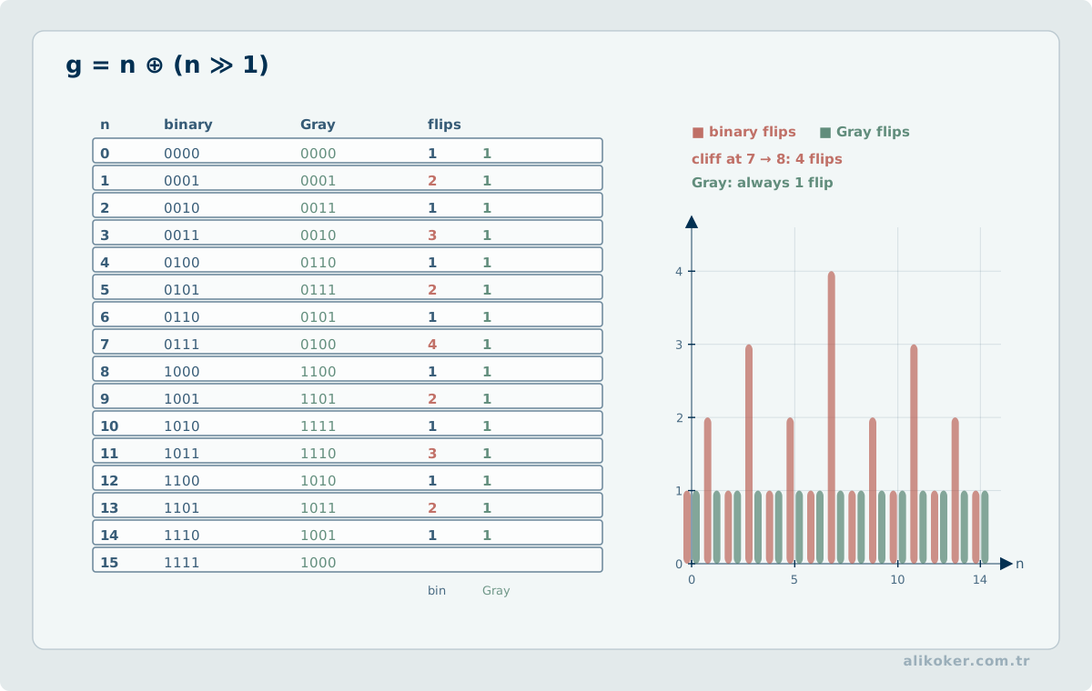
A representation changes the geometry seen by the search algorithm. Two candidate solutions that are close in the problem domain can be far apart in the encoded chromosome, and a one-bit mutation can therefore create either a very small or a very large phenotypic change.

For a binary field of m bits mapped to [a,b], the nominal resolution is

Δ = (b - a) / (2^m - 1).

Resolution alone is not enough. Standard binary coding has Hamming cliffs: adjacent numeric values can differ in many bits. Gray coding reduces that local discontinuity because consecutive code words differ by one bit. It does not make the optimization problem easier in every case, but it can make mutation locality better aligned with the numeric neighborhood.

Representation should therefore be evaluated together with crossover and mutation. A representation that is compact but destroys useful neighborhoods can be worse than a slightly larger representation that preserves problem structure.

1.5. Epistasis and Operator Compatibility

When one variable changes the usefulness of another, the chromosome has epistatic interactions. High epistasis makes simple one-point crossover more likely to break useful combinations. In such problems, linkage-aware operators, real-coded representations, problem-specific crossover, or a different optimizer may be more appropriate.

The engineering question is not whether a chromosome is valid. It is whether the representation makes useful structure reachable under the selected operators.

1.6. Reading Representation, Selection, Variation, and Fitness as One Loop

A genetic algorithm emerges from the interaction of three mechanisms, and most of its behavior can be understood through that interaction.

The population provides parallel sampling. Maintaining multiple candidates at the same time allows the search to accumulate information from different regions of the search space. This is one of the main mechanisms that prevents the search from behaving like a purely single-point local optimizer.

Selection provides exploitation. Better candidates receive more reproductive opportunity, concentrating search effort in promising regions. If selection pressure dominates, however, the population can collapse into near-copies of a small number of individuals and lose useful diversity.

Crossover and mutation provide exploration. Crossover recombines partial structures carried by different individuals, while mutation can reintroduce values or structures that selection and drift have removed. If exploration dominates without sufficient selection pressure, the search approaches random sampling.

The practical design problem is therefore to balance exploitation and exploration. Selection pressure, operator probabilities, population size, elitism, niching, diversity preservation, and island models are different controls on the same underlying trade-off.

Representation is not outside this framework; it is central to it. The encoding determines whether an operator produces meaningful offspring. Standard crossover on a permutation can create invalid solutions, while an unsuitable binary representation of a continuous variable can introduce Hamming cliffs. Both are manifestations of the same design error: the representation and the variation operator do not respect the structure of the problem.

Theoretical results provide useful intuition but not universal success guarantees. The schema theorem and building-block hypothesis explain some mechanisms of propagation and recombination, while Royal Road experiments show that simpler search strategies can outperform genetic algorithms under particular structures. The No Free Lunch result reinforces the broader engineering conclusion: no search method is universally superior. A genetic algorithm is strongest when its representation, operators, constraints, and fitness model are aligned with the structure of the problem.

1.7. Core Design Decisions in a Genetic Algorithm

A genetic algorithm should be treated as an optimization framework with explicit design decisions:

problem definition
→ representation
→ objective and constraints
→ initialization
→ selection pressure
→ variation operators
→ replacement
→ diversity control
→ termination
→ comparison with strong baselines

Reproducible experiments require recording the random seed, implementation version, parameter configuration, stopping rule, and evaluation budget.

Unit 2: Binary-Coded Genetic Algorithms

A conventional cycle is:

initial population
        |
        v
fitness evaluation
        |
        v
selection -> crossover -> mutation
        |                    |
        +------ new generation
                   |
                   +--> stop? -- no --> evaluation
                           |
                          yes
                           v
                         result

define representation and objective
generate initial population
repeat:
    evaluate fitness
    select parents
    recombine
    mutate
    form the next generation
    test termination criteria

For a parameter in [a, u] encoded with m bits, the representable resolution is:

(u - a) / (2^m - 1)

and decoding can be written as:

x = a + integer(bits) * (u - a) / (2^m - 1)

Standard binary coding may create a Hamming cliff: adjacent numerical values can require many simultaneous bit changes. Gray coding avoids this specific discontinuity because adjacent encoded integers differ by one bit.

A binary genetic algorithm starts by defining what a chromosome represents and which bit patterns are feasible. Fitness must align with the objective, with an explicit treatment of constraint violations. Check offspring feasibility after selection, crossover, and mutation. Across generations, monitor not only best fitness but also loss of diversity and sensitivity to random initialization.

2.1. Initialization, Selection, Crossover and Mutation

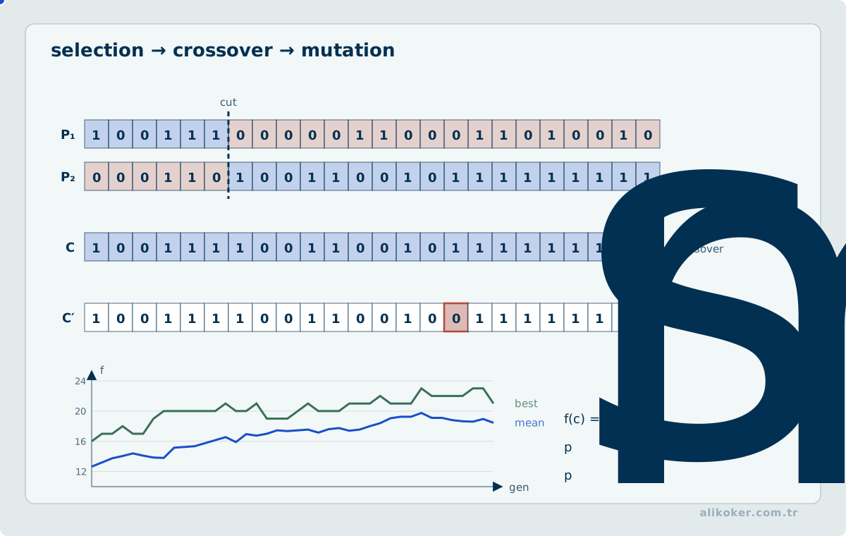
Initialization should provide sufficient diversity without violating hard constraints. Selection creates reproductive pressure toward fitter candidates. Crossover recombines parental material, while mutation introduces local variation and helps prevent irreversible loss of alleles.

Mutation rates that are too low can allow diversity to collapse; rates that are too high can make the process resemble random search. Crossover and mutation therefore cannot be tuned independently from population size, representation, selection pressure, and replacement strategy.

Unit 3: Real-Coded Genetic Algorithms

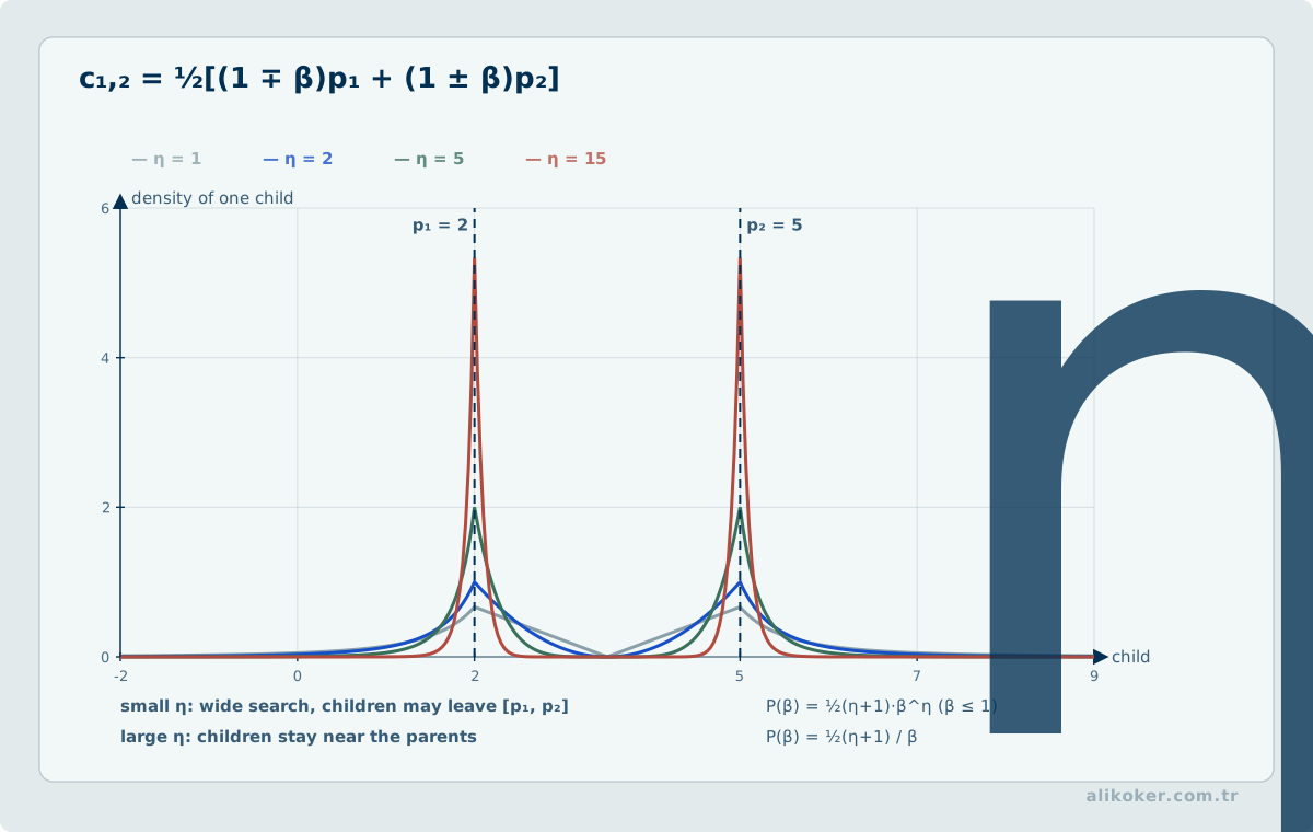
Binary encoding is unnecessary when decision variables are naturally continuous. Real-coded chromosomes represent parameters directly:

x = [x1, x2, ..., xn]

Common recombination operators generate offspring between or around parental values. Mutation may use Gaussian, uniform, polynomial, or adaptive perturbations. Boundary handling must be defined explicitly: clipping, reflection, resampling, repair, or a constraint-aware operator can produce materially different search behavior.

Real-coded optimization starts by defining bounds for decision variables. If crossover or mutation produces out-of-range values, choose an explicit repair, resampling, or penalty policy. With a noisy objective, a single evaluation may misrank individuals and repeated evaluation may be needed. Assess solution quality using distributions across runs and constraint satisfaction, not merely the best value from one generation.

Unit 4: Selection Methods and Selection Pressure

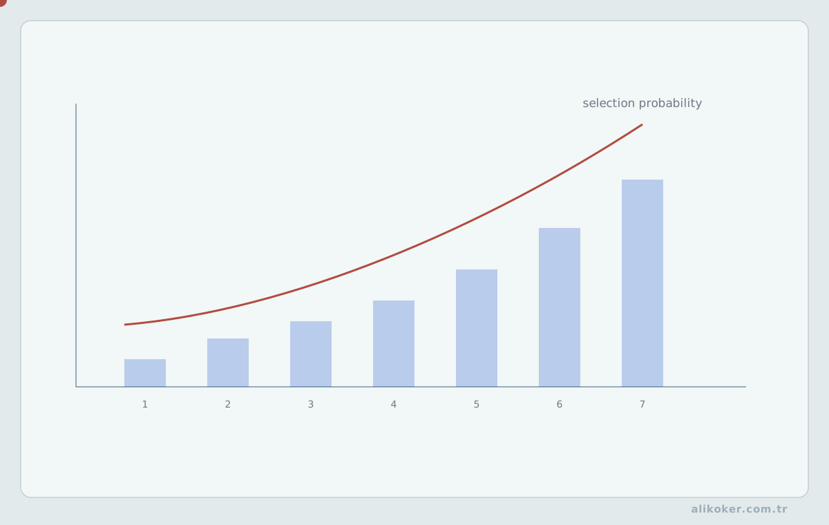
Fitness-proportionate selection assigns probability according to relative fitness, but it is sensitive to scaling and can behave poorly when fitness values are negative or tightly clustered.

low selection pressure            high selection pressure
          |                                |
          v                                v
preserves diversity                faster convergence
slower exploitation                diversity loss
                                   premature convergence risk

Ranking selection operates on order rather than raw magnitude. Tournament selection chooses the best individual from a random subset and provides a simple way to control pressure through tournament size.

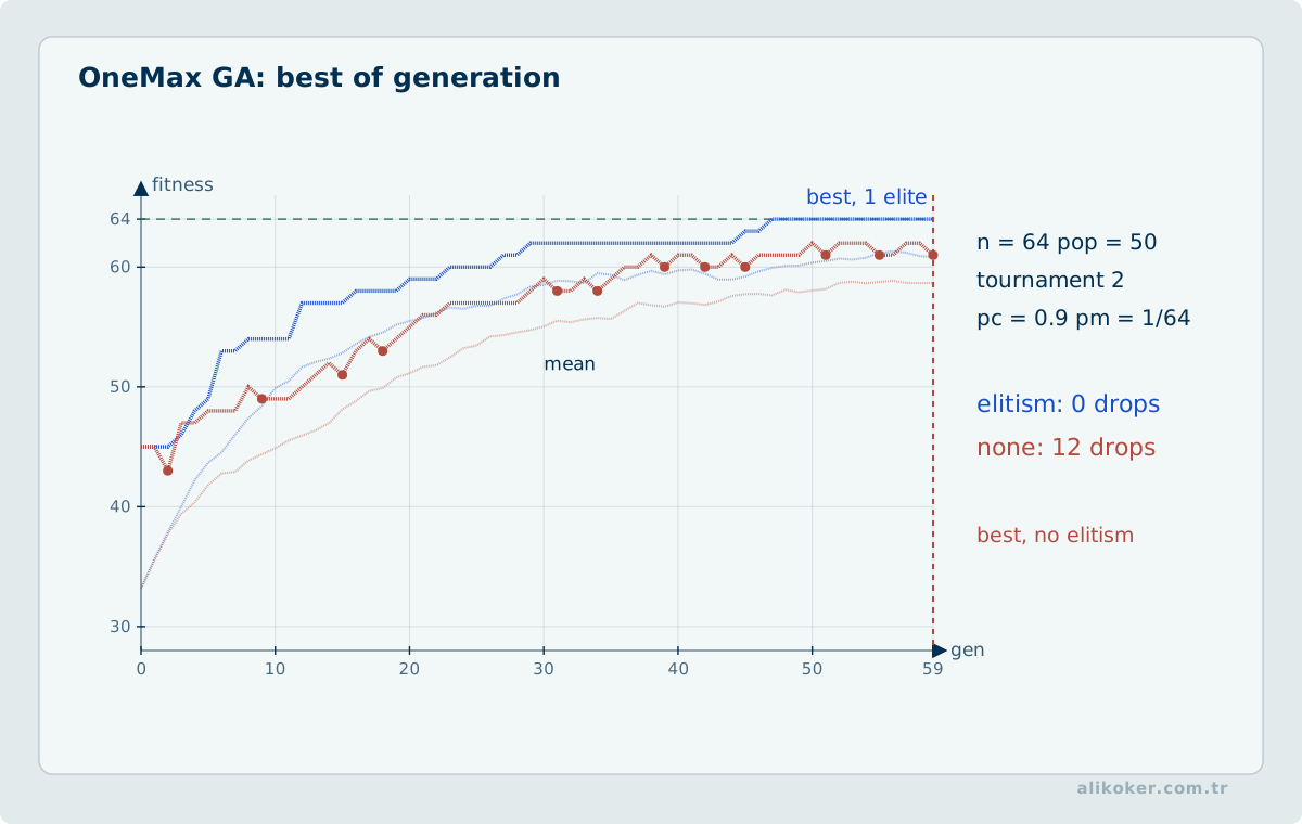
Elitism preserves one or more of the best solutions. It prevents regression of the best-known objective value, but excessive elitism can accelerate premature convergence.

Unit 5: Representation

Representation determines neighborhood structure. Binary strings, integer vectors, real vectors, permutations, trees, and problem-specific structures require different operators.

A representation is effective when small genetic changes tend to produce meaningful changes in the phenotype and when crossover can preserve useful partial structures. Variable interaction, often discussed as epistasis, must therefore be considered together with encoding and operator design.

Unit 6: Parameters, Complexity and Convergence

For population size N, generation count G, and fitness-evaluation cost C(f), the dominant runtime is often approximately:

exploration <---------------------------> exploitation
diversity                                 preserve good candidates
mutation                                  selection / elitism

goal: balance search without collapsing to either extreme

O(G * N * C(f))

In engineering optimization C(f) may represent a finite-element simulation, physical experiment, or other expensive evaluation. In such cases, reducing the number of evaluations matters more than micro-optimizing crossover.

Useful techniques include memoization of repeated candidates, surrogate models, parallel evaluation, early rejection, and adaptive stopping.

Premature convergence occurs when diversity disappears before the population reaches a satisfactory region. Monitoring genotype diversity, phenotype diversity, fitness variance, and improvement rate gives more information than a fixed generation limit alone.

Unit 7: Constraints and Penalty Functions

Constrained problems may be handled through repair operators, feasibility-preserving representations, rejection, ranking rules, or penalty functions.

A penalty formulation can be written as:

F(x) = f(x) + λ * violation(x)

for minimization. The penalty coefficient must balance objective quality against feasibility. A fixed coefficient is simple but can be brittle; adaptive penalties or feasibility-first comparison rules are often more robust.

How a penalty function changes the decision. Consider maximizing f(x) = 12x − x² under x ≤ 5, with 0 ≤ x ≤ 8. The unconstrained maximum occurs at x = 6, which is infeasible. The constrained optimum is x = 5, with f(5) = 35. A quadratic penalty formulation uses F(x) = 12x − x² − ρ·max(0,x−5)². With ρ = 1, the derivative in the infeasible region is F'(x) = 12 − 2x − 2(x−5) = 22 − 4x, giving a penalized optimum at x = 5.5. Despite the penalty, this solution still violates the original constraint. Increasing the penalty weight reduces violation but may distort the search landscape; a finite quadratic penalty does not generally enforce exact feasibility. A genetic algorithm using this objective therefore needs an explicit feasibility check, repair operation, or feasibility-first comparison policy when producing the final result.

7.1. Distinguishing Feasibility Repair from Penalty Functions

In constrained optimization, the objective \(f(x)\) and feasible region \(\mathcal F=\{x:g_j(x)\leq0\}\) are separate concepts. A penalty method alters candidate ranking by quantifying violations; a repair operator attempts to transform a candidate into \(R(x)\in\mathcal F\). Their effects on the search space differ. A fixed large penalty can dominate objective quality, whereas a small penalty can allow infeasible candidates to dominate the population.

For a binary selection vector with a weight bound \(W\), one penalty is \(\lambda\max(0,\sum_i w_i x_i-W)\). A repair operator could remove selected items until the bound is met. The removal rule, however, biases search toward certain solutions; repair is not neutral. When maintaining elitism and diversity among feasible candidates, duplicates created by repair should also be monitored.

Reports should include not only the best objective value but the feasibility rate, objective-evaluation budget, repair cost, and outcome distribution across independent runs. A representation that preserves feasibility by construction may avoid much of the penalty or repair overhead, but it also changes the neighborhood reachable by crossover and mutation.

Unit 8: Combinatorial Problems and Permutations

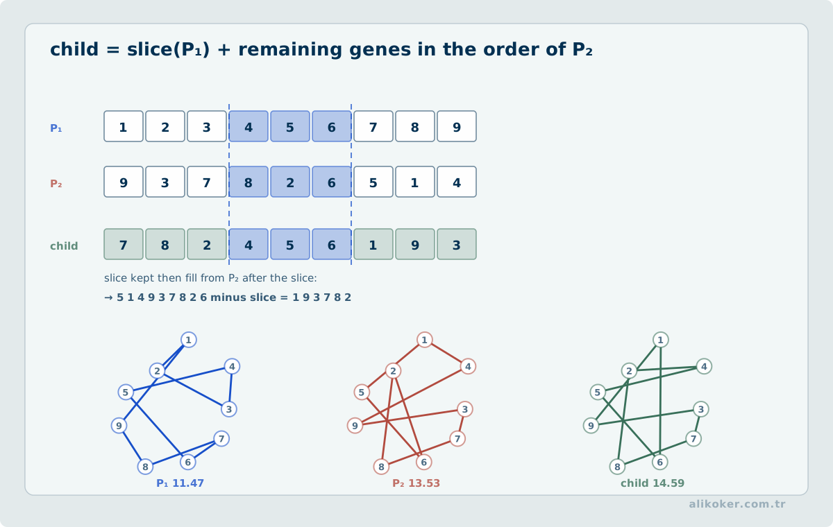
For problems such as the Traveling Salesperson Problem, a chromosome is often a permutation. Ordinary one-point crossover can create duplicate cities and omit others, so permutation-specific operators are required.

Examples include partially matched crossover, order crossover, cycle crossover, swap mutation, insertion mutation, and inversion mutation. The representation should preserve the invariant that every element appears exactly once.

8.1. Pareto Dominance and Population Diversity

Multi-objective optimization does not normally produce one scalar optimum. A solution is Pareto-dominated if another solution is no worse in every objective and strictly better in at least one. The non-dominated set approximates the Pareto front.

Algorithms such as NSGA-II combine two pressures:

• move the population toward non-dominated regions,
• preserve diversity along the front.

A common mechanism is non-dominated sorting followed by a crowding-distance estimate. Selection then prefers better Pareto rank and, within the same rank, less crowded regions.

A result should therefore not be reported as “the best chromosome” unless an explicit preference function has reduced the objectives to one scalar decision. For a genuine multi-objective problem, the report should include the objective definitions, the final non-dominated set, the diversity criterion, the random seeds, and the number of objective evaluations.

Unit 9: Theoretical Foundations

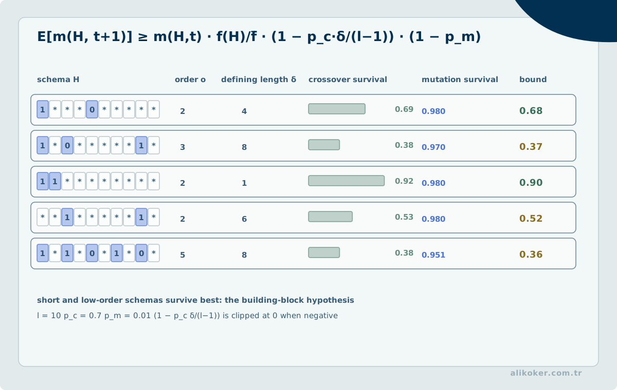
Schema theory studies subsets of strings sharing patterns at selected positions. Holland's schema theorem describes expected propagation of short, low-order, above-average schemata under simplified assumptions. It is historically important, but it should not be treated as a complete explanation of modern genetic-algorithm behavior.

The No Free Lunch results establish that, averaged uniformly over all possible objective functions, no optimizer is universally superior. Practical performance therefore comes from matching algorithmic bias to problem structure.

Deceptive functions, Royal Road functions, building-block hypotheses, linkage, and exact population models are useful for studying when recombination helps or fails.

Unit 10: Applications

Genetic and evolutionary methods are used in engineering design, scheduling, parameter estimation, control, feature selection, strategy search, symbolic program evolution, neural architecture or parameter evolution, and multi-objective optimization.

The correct engineering question is not whether a genetic algorithm can encode the problem, but whether it reaches solutions of sufficient quality with acceptable evaluation cost compared with deterministic optimization, local search, mixed-integer programming, Bayesian optimization, differential evolution, CMA-ES, or problem-specific heuristics.

10.1. Comparing Multiobjective Drive Tuning under the Same Experiment Budget

When a genetic algorithm selects speed-controller gains Kp and Ki, fitness should not be reduced to tracking error alone. For example, J1 = ∫|e(t)|dt measures accumulated tracking deviation, J2 = ∫i(t)²dt is a proxy for current-related thermal loading, and J3 = max(0, overshoot - allowed_overshoot) captures a constraint violation. These objectives have different units; combining them with arbitrary weights can conceal the underlying engineering tradeoff. Unacceptable current or overshoot should often be treated as feasibility boundaries rather than preferences that may be traded away.

Each candidate must be tested against the same load profiles, initial conditions, and observation horizon. Under stochastic disturbances, repeat evaluations should be used instead of selecting a candidate on its luckiest run. With an identical computational budget, the evolutionary approach can be compared against a grid search, local optimization, or defensible model-based initial gains. A Pareto set reveals alternatives between error and energy; final deployment still depends on physical limits, reliability, and maintenance requirements.

Unit 11: Evolution as a Modeling Tool

Evolutionary algorithms can also be used as computational models. Co-evolution, sexual selection, ecological competition, learning-evolution interaction, and evolving cellular automata allow hypotheses about adaptive systems to be tested in controlled simulations.

Such simulations are models, not direct evidence that biological evolution follows the same simplified computational rules.

Unit 12: Related Evolutionary Methods

12.1. Differential Evolution

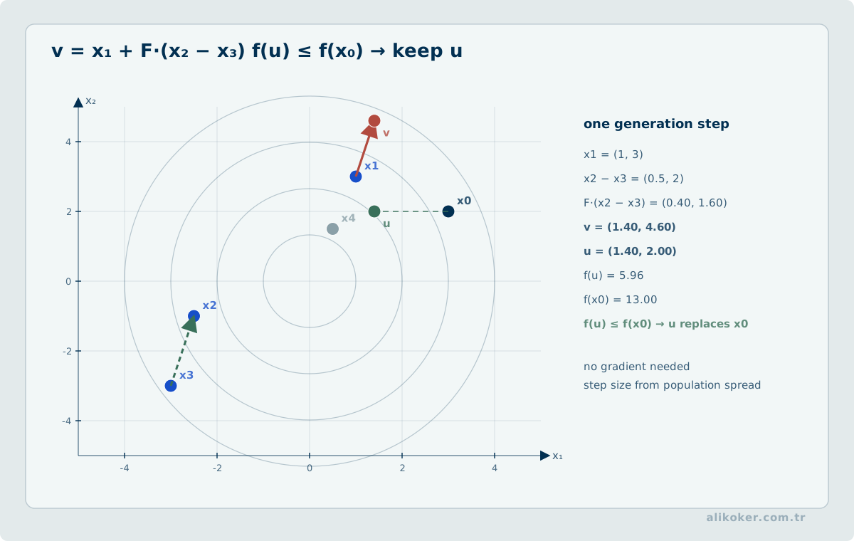
Differential Evolution constructs trial vectors from scaled differences between population members. It is especially effective for many continuous black-box optimization problems and requires no binary encoding.

12.2. CMA-ES

Covariance Matrix Adaptation Evolution Strategy adapts a multivariate search distribution. The covariance matrix learns correlations between variables, allowing the search distribution to rotate and stretch according to the local landscape.

12.3. Multi-objective Optimization

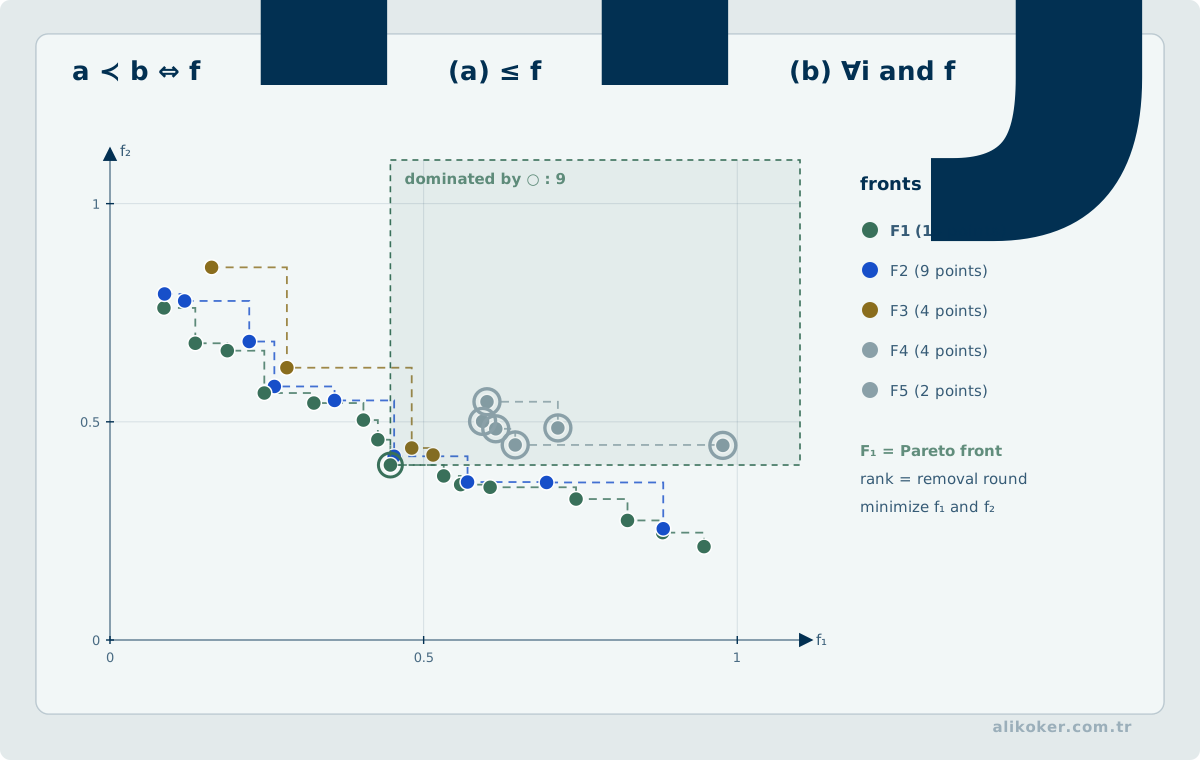
When objectives conflict, a single optimum may not exist. The relevant solution set is the Pareto front: solutions for which no objective can be improved without worsening at least one other objective.

12.4. Optimizing Thresholds and Weights in Analytical Systems

A genetic algorithm can tune thresholds or weights in an analytical system, but only after "good" behavior has a measurable definition. Maximizing the system's own anomaly or network score is not a sufficient fitness function. False positives, false negatives, analyst workload, computational cost, and stability may all matter.

A candidate can be represented as:

C = [anomaly_threshold,
     time_window,
     similarity_threshold,
     weight_1,
     weight_2]

Instead of forcing everything into one objective, a multi-objective problem can use:

minimize false_positive_rate
minimize false_negative_rate
minimize analyst_workload
minimize compute_cost
maximize stability

These goals will often conflict. A Pareto frontier makes the trade-off explicit—for example, how much additional false-positive rate and review workload must be accepted to gain recall. The value of the GA is therefore not that it discovers a magical threshold, but that it explores a clearly defined trade-off surface.

Fitness quality is a hard boundary. Without expert-validated cases, synthetic scenarios with known outcomes, or another defensible ground truth, using the system's own score as fitness becomes circular:

the system produces a score
        ↓
the GA maximizes that score
        ↓
the result receives a higher score

Nothing in this loop establishes better real-world performance.

Optimization and validation data should also be separated. If thresholds are chosen and reported on the same records, the thresholds themselves can overfit:

optimization corpus != validation corpus

Whenever possible, validation should be separated by time, source, or case. Distribution shift in deployment can invalidate a previously good Pareto solution and requires renewed measurement.

For a handful of smooth or directly searchable parameters, a genetic algorithm is usually not the first choice. Grid search, binary search, convex/linear optimization, or domain knowledge can be cheaper and more reproducible. Evolutionary search becomes more defensible when the space is large, irregular, mixed discrete/continuous, non-differentiable, and genuinely multi-objective. Selecting the optimizer is itself part of the engineering problem.

12.5. The Role of Evolutionary Optimization in Artificial Intelligence

12.6. Evolving Artificial Neural Networks

Weight evolution with a fixed architecture: weights can be encoded in a chromosome and fitness can be derived from model error or task return. The method does not require differentiability, but typically needs far more evaluations than gradient training and does not scale competitively to large networks by default.

Architecture evolution: layer and connection structure can itself be searched. Direct encodings grow rapidly with network size, while indirect encodings can express repeated or modular structure more compactly. The representation determines which architectures are easy or difficult for evolution to discover.

This illustrates a general principle: the genotype-to-phenotype mapping shapes the effective search space. Compact structural encodings can improve regularity, while reducing the ability to tune every connection independently.

12.7. Conditions Favoring Derivative-Free Search

A genetic algorithm does not require derivatives of the objective. This is useful for simulators, discrete choices, non-differentiable rules, and black-box objectives. The cost can be high when every fitness evaluation is expensive because population-based search requires many evaluations.

In machine learning, genetic algorithms are therefore often more useful as an outer optimization layer than as a replacement for every training algorithm:

feature subset
hyperparameters
architecture / rule structure
multi-objective tradeoff

The outer design may evolve while model weights are trained by a more efficient gradient method.

12.8. Neuroevolution and Policy Search

When gradient information is weak or unavailable, policy parameters can be evolved directly. Fitness may represent total episode performance. Such methods parallelize naturally, but sample efficiency can be lower than gradient-based alternatives.

12.9. Multi-objective AI Design

Production models are rarely selected by accuracy alone. Latency, memory, energy, and model size can be competing objectives. Multi-objective evolutionary optimization can expose a Pareto frontier rather than hiding these tradeoffs in one arbitrary score.

The modern role of genetic algorithms is therefore not to evolve every neural network. They remain a strong black-box optimization method when gradients are unavailable or when external design choices must be searched jointly.

12.10. Particle Swarm Optimization Is Not a Genetic Operator

Each particle in PSO has a position x_i and velocity v_i. A standard update is v_i <- ωv_i+c1 r1(p_i-x_i)+c2 r2(g-x_i), then x_i <- x_i+v_i. Here p_i is the particle's personal best and g is the neighborhood or global best under the chosen topology. This is not GA crossover or mutation. Inertia ω, attraction constants, random factors, velocity clipping, and boundary-handling rules shape exploration and convergence.

For comparisons among PSO, GA, and differential evolution, equal objective-function evaluation counts are generally more meaningful than equal iterations. Record multiple starting seeds, failures, median final fitness, and interquartile range. A quantum-inspired swarm implemented on classical hardware does not thereby establish a physical quantum speedup.

Unit 13: Multi-Objective Quality, Noisy Fitness, and Experimental Design

The engineering quality of a genetic algorithm is not determined only by whether one run finds a strong candidate. Stability across independent runs, uncertainty in the fitness function, use of the evaluation budget, and the quality of the Pareto set are part of the result.

13.1. Measuring Pareto-front Quality

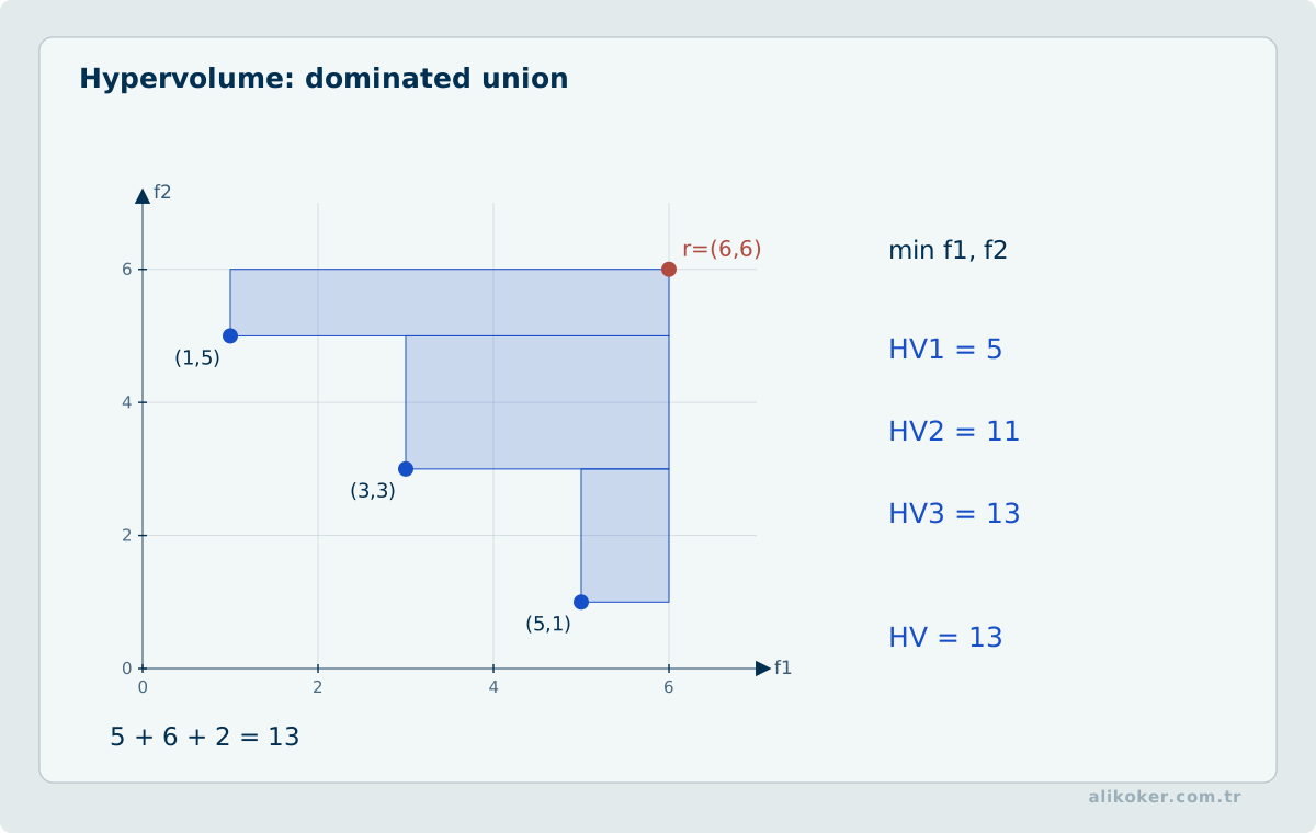
In multi-objective optimization, simply counting non-dominated solutions is insufficient. Two algorithms may return the same number of solutions while one is closer to the useful Pareto region and covers the trade-off surface more evenly.

Hypervolume measures the objective-space volume dominated by the returned Pareto set relative to a chosen reference point. It combines convergence and spread, but its value depends on objective scaling and the reference point. Those choices must therefore remain fixed when experiments are compared.

When a reference Pareto front is known, synthetic benchmarks can also use measures such as generational distance. In real engineering problems the true front is usually unknown, so hypervolume, coverage, spread, and domain-specific decision criteria should be interpreted together rather than as interchangeable absolute scores.

13.2. Noisy Fitness Functions

If fitness comes from simulation, physical experimentation, sampling, or another stochastic algorithm, repeated evaluation of the same chromosome can produce different values. Selection based on a single sample can therefore rank candidates incorrectly because of measurement noise rather than solution quality.

Depending on cost, useful strategies include:

• evaluating the same candidate repeatedly and using a mean, median, or selected quantile,
• allocating extra evaluations to candidates near a selection boundary,
• using common random numbers so competing candidates are evaluated under matched stochastic scenarios.

The goal is not necessarily to eliminate noise. It is to control uncertainty in the selection decision. Adaptive resampling can spend additional evaluations only where the ranking is genuinely ambiguous.

13.3. Evaluation Budget as a Common Currency

Generation count is not a sufficient basis for comparing evolutionary algorithms. Two runs with different population sizes may use radically different numbers of objective-function calls even when both execute the same number of generations.

At minimum, report these costs separately:

number of objective evaluations
wall-clock time
processor / accelerator resources used

Parallel evaluation may reduce wall-clock time without reducing total computation. In an asynchronous evolutionary algorithm, candidates that finish earlier may influence selection earlier, so timing can change algorithmic behavior. The update and selection policy therefore belongs to the experimental contract.

13.4. Stopping Criteria and Reproducibility

A fixed generation limit is simple but does not describe convergence quality. Practical stopping criteria may combine an evaluation budget, a target objective value, a no-improvement window, or a diversity threshold.

A reproducible experiment should preserve the random-number generator and seed, population size, operators and parameters, stopping rule, evaluator version, constraint-handling policy, and benchmark or simulation scenario. The best result from one stochastic run is not an estimate of general algorithm performance.

13.5. Report Distributions, Not a Single Run

Genetic algorithms are stochastic. One seed and one best result do not characterize the method. Independent runs should report central tendency, spread, and failure rate.

Comparisons should also use comparable compute budgets. A method using many more fitness evaluations should not be judged only by its final score.

Convergence analysis should track population diversity as well as the best individual; collapsing diversity with a stagnant best score is a warning sign for premature convergence.

13.6. Reporting Stochastic Optimization Results

One genetic-algorithm run is not a result distribution. Independent seeds should report central tendency, spread, worst cases, and the fraction of runs that fail to reach the target.

Algorithms should be compared under equivalent compute budgets. Total fitness evaluations or measured runtime can be more meaningful than population size or generation count alone.

Population diversity should be monitored alongside the best score. Early collapse can indicate parameter or representation problems. Where possible, comparisons should include a classical method or a simple baseline.

13.7. Representation and Fitness Must Be Designed Together

In a genetic algorithm, chromosome representation is more than a storage format; it also defines the neighbourhood structure of the search space. Encoding the same problem as a bit string, integer sequence, permutation, or real-valued vector changes the candidates produced by crossover and mutation. In permutation problems in particular, an ordinary one-point crossover can create invalid repetitions, so the operator has to respect the constraints of the representation.

The fitness function is likewise an approximation of the real objective. If an easily measured proxy is chosen, the algorithm may optimize that proxy very successfully while moving away from the engineering goal that actually matters. Adding every constraint as a very large penalty can also distort the search landscape. Repair operators, constraint-preserving representations, or feasibility-aware operators may be more natural for some problems.

Selection pressure that is too weak spreads useful information slowly; pressure that is too strong can remove diversity and cause premature convergence. Mutation is not merely a way to “add randomness.” It can restore variation lost from the population, but excessive mutation makes directed search approach random exploration.

For this reason, a stochastic optimizer should not be evaluated from one fortunate run. Repeated runs with different random seeds should expose the median, distribution, and failure cases. The result of a genetic algorithm is therefore not only the best fitness value found; it is the behaviour of the complete representation + operators + selection + randomness + stopping rule system.

13.8. Robustness under Noisy Fitness Functions

Robust statistics asks how much an estimator degrades under small departures from an idealized model. For genetic-algorithm experiments, reporting the median and MAD across independent runs exposes variability that a single best fitness value hides; influence functions and breakdown points further show how easily a performance summary can be distorted by a few exceptional runs. In heavy-tailed or contaminated data, decisions based only on the mean and standard deviation can be misleading.

• Use repeated evaluation or robust summaries when fitness measurements are noisy.
• Measure the risk of a single extreme fitness value steering the population incorrectly.
• Keep parallel evaluation speed separate from selection pressure.

13.9. Selection Bias under Noisy Fitness

A chromosome receiving a high score in one stochastic evaluation has not necessarily achieved a superior expected fitness. Selecting the maximum observed score among many candidates preferentially selects positive noise excursions. Fitness may therefore be estimated from independent replications such as f̂(x) = (1/m) Σ(j=1..m) f(x,ω_j). When evaluation time is limited, it can be more useful to allocate extra replications to promising candidates with overlapping uncertainty than to assign the same replication count to every individual.

Evaluating competing chromosomes under common random scenarios may reduce variance in their difference. The intended role of fixed scenarios across generations must be stated: repeatedly optimizing on the same finite scenario set can overfit that set and exaggerate performance on the actual input distribution. The selected final candidate requires a fresh, independent scenario-based assessment.

13.10. Heuristic Search and Convergence Guarantees

Genetic algorithms can find useful solutions in large, discrete search spaces, but the best surviving individual does not prove attainment of a global optimum. Asymptotic results for particular evolutionary schemes do not guarantee a specified rate or success probability under a finite budget. Comparisons should report an equal number of objective-function evaluations, multiple independent runs, distributions of solution quality and a clear stopping rationale. Parallel fitness evaluation may reduce elapsed time without reducing the number of evaluations required by the search.

References

• Mor Harchol-Balter. Performance Modeling and Design of Computer Systems: Queueing Theory in Action. Cambridge University Press, 2013.

• Peter J. Huber; Elvezio M. Ronchetti. Robust Statistics. 2nd ed. Wiley, 2009.

• Çunkaş, M. Genetik Algoritmalar ve Uygulamaları Ders Notları. Selçuk University, Faculty of Technical Education, Department of Electronics and Computer Education, Spring 2006.

• Deb, K.; Pratap, A.; Agarwal, S.; Meyarivan, T. “A Fast and Elitist Multiobjective Genetic Algorithm: NSGA-II.” IEEE Transactions on Evolutionary Computation, 6(2), 182-197, 2002. https://doi.org/10.1109/4235.996017

• Eiben, A. E.; Smith, J. E. Introduction to Evolutionary Computing. Springer.

• Goldberg, D. E. Genetic Algorithms in Search, Optimization, and Machine Learning. Addison-Wesley, 1989.

• Hansen, N.; Ostermeier, A. “Completely Derandomized Self-Adaptation in Evolution Strategies.” Evolutionary Computation, 9(2), 159-195, 2001. https://doi.org/10.1162/106365601750190398

• Holland, J. H. Adaptation in Natural and Artificial Systems. University of Michigan Press, 1975.

• Mitchell, M. An Introduction to Genetic Algorithms. MIT Press, 1996.

• Stanley, K. O.; Miikkulainen, R. “Evolving Neural Networks through Augmenting Topologies.” Evolutionary Computation, 10(2), 2002. https://doi.org/10.1162/106365602320169811

• Storn, R.; Price, K. “Differential Evolution – A Simple and Efficient Heuristic for Global Optimization over Continuous Spaces.” Journal of Global Optimization, 1997.

• Walter W. Piegorsch, Richard A. Levine, Hao Helen Zhang, Thomas C. M. Lee (eds.). Computational Statistics in Data Science. Wiley, 2022. ISBN 9781119561071.
• Naveenkumar, P.; Sharma, V.; Devarajan, G.; Abdullah, A.; Elngar, A. A. (eds.). Handbook of AI-Based Mechatronics Systems and Smart Solutions in Industrial Automation. CRC Press, 2026. DOI: https://doi.org/10.1201/9781032615790.
• Chunwei Zhang, Tianpeng Li, Ying Dai, Li Sun, and Ardashir Mohammadzadeh. Practical Neural Networks in Python and MATLAB. Springer Nature, 2026. DOI: https://doi.org/10.1007/978-3-032-14746-2.