Artificial Neural Networks and Learning Models

My neural-network notes from the 2013-2015 period were centered on perceptrons, multilayer networks, backpropagation, LVQ, ART and Elman networks. I preserve that historical core. CNNs, LSTM/GRU, attention, Transformers and generative models are later technical additions rather than concepts retroactively attributed to the original course notes, and I keep that distinction visible.

Unit 1: Artificial Intelligence and Machine Learning

Artificial intelligence

Artificial intelligence is a broad field concerned with computational systems that perform tasks associated with perception, reasoning, learning, planning, language, decision-making or adaptive behavior.

AI is not synonymous with neural networks. Symbolic reasoning, search, probabilistic models, optimization, expert systems, evolutionary computation and machine learning all belong to the wider field.

Application areas

Applications include:

• classification and pattern recognition,
• forecasting,
• control and optimization,
• speech and image processing,
• anomaly detection,
• decision support,
• robotics,
• natural-language processing.

The suitability of a method depends on the data, required guarantees, latency, interpretability, resource budget and error cost.

Machine learning

Machine learning constructs a model from data rather than expressing every decision rule explicitly.

A generic supervised-learning problem can be written as a set of input-output examples:

D = {(x_i, y_i)}

and a parameterized model:

y_hat = f(x; theta)

Training selects parameters theta to reduce an objective measured on examples while retaining the ability to generalize to unseen data.

Learning types

Supervised learning uses labeled examples containing target values/classes.

Unsupervised learning uses data without explicit target labels to discover structure, density, clusters or representations.

Reinforcement learning learns behavior through interaction and reward signals rather than a fixed label for every action.

Semi-supervised and self-supervised methods combine or derive supervision in other ways.

Hetero-association and auto-association

An auto-associative model learns to reproduce or recover a representation related to its input:

x -> x

A hetero-associative model maps one pattern to a different associated target:

x -> y

These concepts appear historically in associative-memory neural models and still provide a useful way to distinguish reconstruction from cross-pattern mapping.

Learning paradigms and strategies

Learning may update parameters:

• online, after individual examples,
• in mini-batches,
• in full batches,
• competitively,
• through error correction,
• through correlation/Hebbian-style rules.

The algorithm must specify not only the model but also how examples are selected, how errors are computed, how parameters are initialized and when training stops.

Unit 2: Introduction to Artificial Neural Networks

Basic idea

An artificial neural network is a parameterized composition of simple processing units. A unit commonly computes a weighted sum followed by an activation function:

z = sum(w_i x_i) + b

y = phi(z)

The weights determine how inputs contribute to the unit. Training modifies weights and biases according to an objective or learning rule.

Biological analogy

The historical terminology is inspired by neurons, synapses and activation, but an artificial neuron is a mathematical abstraction. A modern neural network should not be interpreted as a faithful simulation of biological nervous tissue.

Training, validation and test

Data should be separated according to purpose:

• training data update model parameters,
• validation data guide model/hyperparameter selection and stopping,
• test data estimate final generalization after design decisions are complete.

Repeatedly tuning against the test set leaks test information into the design and invalidates its role as an independent estimate.

Adaptation and generalization

A model that only reproduces its training examples has not necessarily learned a useful function. Generalization is performance on data not used to fit the parameters.

The achievable generalization depends on:

• data quality and representativeness,
• model capacity,
• regularization,
• optimization,
• distribution shift,
• label noise,
• evaluation design.

Historical development

Important milestones include the McCulloch-Pitts formal neuron, Rosenblatt's perceptron, ADALINE/MADALINE, multilayer networks trained with backpropagation, recurrent networks and later deep-learning architectures.

The historical period matters. The 2013-2015 notes were written when CNNs and recurrent networks were already established and deep learning was rapidly expanding, but Transformer architectures did not yet exist. Later sections explicitly identify post-2015 additions.

Distributed representation

Knowledge in a neural network is generally distributed across parameters rather than stored as one explicit rule per concept. This can provide graceful behavior and representation capacity, but makes explanations harder than in a transparent rule system.

Noise and incomplete data

Neural networks can be robust to noisy inputs when trained for the relevant distribution. Robustness is not automatic. Adversarial inputs, missing values, out-of-distribution samples and sensor failures can still cause confident errors.

Explainability

Model inspection may use feature attribution, activation analysis, surrogate models or domain-specific probes. These techniques provide evidence about behavior but do not convert a complex model into a fully transparent causal explanation.

Limitations

Neural networks can require substantial data and compute, may overfit, can encode dataset bias, and do not inherently provide formal safety guarantees. In critical systems, model accuracy must be combined with validation, monitoring, deterministic preprocessing and system-level controls.

Unit 3: Network Structure and Basic Elements

Processing of a neuron

For input vector x, weights w and bias b:

z = w^T x + b

and output:

y = phi(z)

The model becomes nonlinear when nonlinear activation functions are used between affine layers.

Activation functions

Historical functions include:

• hard threshold/sign,
• linear,
• sigmoid,
• hyperbolic tangent.

Modern networks also use ReLU and variants:

ReLU(x) = max(0, x)

Sigmoid maps to (0, 1) and is useful for binary-probability outputs under the appropriate loss; tanh maps to (-1, 1). Saturating activations can produce small gradients in deep networks.

Layers

A feed-forward network contains input representation, one or more hidden layers and output layer. A layer's role depends on architecture; the "input layer" may simply denote supplied features rather than trainable neurons.

Model families

Network topology can be:

• feed-forward,
• recurrent,
• convolutional,
• competitive/self-organizing,
• associative,
• energy-based,
• attention-based in later architectures.

The learning rule and network topology are separate dimensions.

Unit 4: Early Neural Networks

Single-layer networks

A single-layer linear threshold classifier forms a decision boundary:

w^T x + b = 0

It can separate linearly separable classes but cannot represent arbitrary nonlinear classification boundaries.

Perceptron

For binary targets and a misclassified example, a classic perceptron update has the form:

w <- w + eta (target - output) x

under one common coding convention.

The perceptron convergence theorem guarantees convergence in finite updates when the training set is linearly separable and assumptions are met. It does not guarantee convergence for non-separable data.

XOR limitation

XOR cannot be separated by one linear decision boundary. This illustrates the limitation of a single-layer perceptron and motivates hidden layers/nonlinear feature transformations.

ADALINE

ADALINE uses a linear activation during learning and adjusts weights to reduce a mean-squared error criterion, historically through the Widrow-Hoff/LMS rule.

A basic gradient form is:

w <- w - eta * dL/dw

The update direction must follow the derivative of the defined loss; notation should not obscure the sign convention.

MADALINE

MADALINE combines multiple ADALINE units. It is historically important as an early multilayer adaptive architecture, although its training methods differ from contemporary generic backpropagation.

Unit 5: Supervised Learning and the Multilayer Perceptron

Multilayer perceptron

An MLP composes affine transformations and nonlinear activations:

h = phi(W1 x + b1)
y_hat = psi(W2 h + b2)

With sufficient hidden capacity and suitable activations it can represent nonlinear decision functions that a single linear layer cannot.

Solving XOR

A hidden layer can construct intermediate regions/features that separate XOR. The important lesson is not a particular hand-coded weight set but that composition of nonlinear units changes the representable function class.

Forward propagation

A feed-forward pass computes layer outputs in order. For layer l:

z^(l) = W^(l) a^(l-1) + b^(l)
a^(l) = phi(z^(l))

The output and target define a loss.

Backpropagation

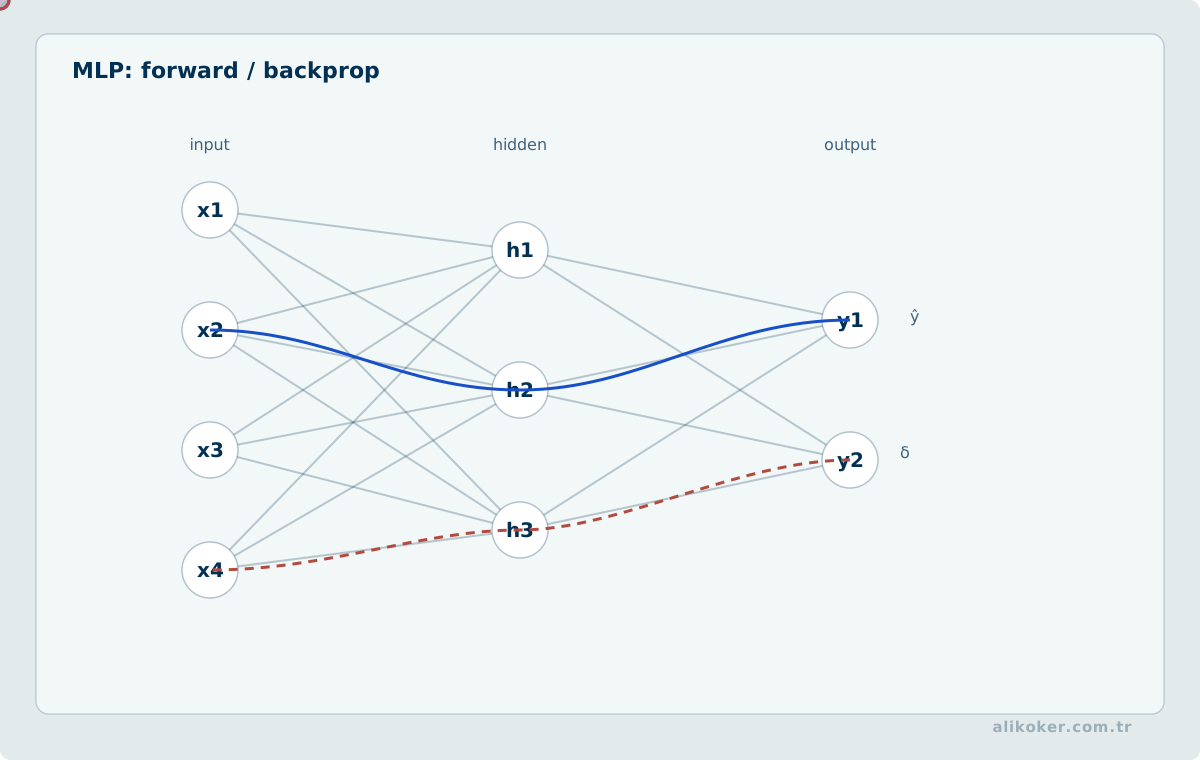
Backpropagation applies the chain rule to compute derivatives of the loss with respect to each parameter efficiently.

For output error signal delta^(L), a hidden-layer error is propagated conceptually as:

delta^(l) = (W^(l+1)^T delta^(l+1)) .* phi'(z^(l))

and weight gradient:

dL/dW^(l) = delta^(l) a^(l-1)^T

Gradient descent then updates parameters:

W <- W - eta * dL/dW
b <- b - eta * dL/db

The exact output delta depends on activation and loss. For example, softmax with cross-entropy leads to a particularly simple derivative under standard formulation.

Training procedure

A practical training loop is:

1. initialize parameters,
2. select a batch/example,
3. perform forward propagation,
4. compute loss,
5. backpropagate gradients,
6. update parameters,
7. evaluate validation behavior,
8. stop according to a defined criterion.

Randomizing/shuffling training examples can reduce systematic ordering effects in stochastic methods.

Error surfaces

Neural-network objectives are generally non-convex. Saddle points, flat regions and different local minima can occur. The goal of optimization is useful generalization, not necessarily discovery of one globally unique parameter vector.

Unit 6: MLP Design and Performance

Performance measurement

A loss used for optimization is not necessarily the only evaluation metric. Classification may require accuracy, precision, recall, F-score, ROC/PR analysis or calibrated error costs. Regression may use MAE, MSE/RMSE or domain-specific tolerances.

Metrics must be selected from the operational consequence of errors.

Overfitting

Overfitting occurs when the learned model captures training-specific noise/patterns that do not generalize. Symptoms include improving training error while validation error stops improving or worsens.

Controls include:

• more representative data,
• regularization,
• early stopping,
• appropriate capacity,
• augmentation where semantically valid,
• cross-validation for limited datasets.

Example selection

Training examples should cover the expected deployment distribution. Random train/test splitting can be misleading when samples from the same subject, session, machine or time period leak correlated information across splits.

Input and output representation

Input scale and encoding directly affect optimization. Categorical variables, bounded numerical measurements, images and time series require different representation choices.

Outputs should match the task: linear outputs for unconstrained regression, logistic-style outputs for binary probabilities, softmax-like normalized outputs for mutually exclusive classes, or structured outputs for more complex tasks.

Weight initialization

Initializing every hidden weight identically prevents symmetry breaking. Random initialization with variance scaled to layer fan-in/fan-out improves signal/gradient propagation. Later Xavier/Glorot and He-style initializations formalize this principle for common activation families.

Learning rate and momentum

A learning rate that is too large can destabilize training; one that is too small can make optimization impractically slow.

Classical momentum accumulates a velocity-like term so updates retain direction across iterations and can smooth oscillation:

v_t = beta v_(t-1) + gradient_term
w_t = w_(t-1) + v_t

with sign convention determined by the update definition.

Scaling

Features with very different numeric ranges can create poorly conditioned optimization. Standardization or bounded scaling should be fit using training data only and then applied consistently to validation/test/deployment data.

Stopping criteria

Training can stop after:

• a maximum epoch count,
• objective convergence,
• validation-based early stopping,
• reaching a domain performance target.

Stopping because training error is nearly zero is not automatically desirable.

Hidden layers and units

There is no universal formula for the correct number of hidden units. Capacity should be selected empirically against data scale, validation behavior, latency/memory constraints and regularization.

Constructive methods grow a network; pruning methods remove weak parameters/units. Modern architecture search and sparsification extend these ideas but do not eliminate the need for independent evaluation.

Unit 7: MLP for Industrial Prediction

Problem definition

An industrial prediction problem begins with a measurable target and a clear decision/use of the prediction. Sensor variables should be selected for causal/operational relevance, not simply because they are available.

Experimental design

If training data come from controlled experiments, the experiment must span the operating region in which the model will later be used. A network cannot be expected to interpolate reliably into regions that are absent or poorly sampled, and extrapolation is especially risky.

Inputs and outputs

Inputs may include process settings, environmental measurements and lagged state. Outputs may represent quality, energy, yield or another process variable.

Leakage must be prevented: a feature that becomes available only after the target event cannot be used for real-time prediction even if it produces excellent retrospective accuracy.

Optimization through a learned model

A trained model can be used as a surrogate inside an optimization loop, but an optimizer may exploit model errors and drive inputs toward unsupported regions. Input constraints and validation against the physical process are therefore necessary.

Unit 8: Learning Vector Quantization

Purpose

LVQ is a prototype-based supervised classification family associated with Kohonen. Each prototype/codebook vector represents a region and carries a class label.

Structure and distance

Given input x, the closest prototype under the chosen metric is found:

c = argmin_j ||x - w_j||

The winning prototype determines the class.

LVQ1 update

A common LVQ1 rule moves the winning prototype toward a correctly classified sample:

w_c <- w_c + alpha (x - w_c)

and away from a sample of another class:

w_c <- w_c - alpha (x - w_c)

The learning rate is commonly reduced over training.

Decision regions

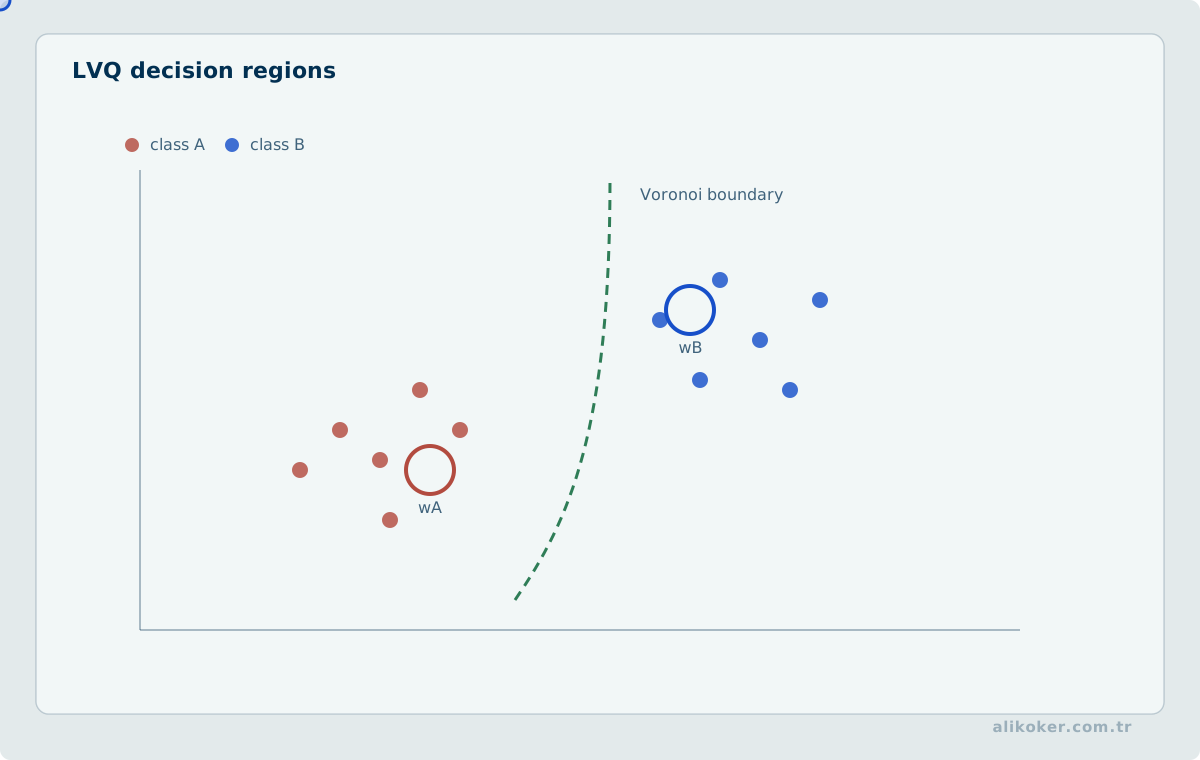
Nearest-prototype classification partitions feature space into Voronoi-like regions. The quality therefore depends strongly on feature scaling, distance metric and prototype placement.

LVQ2 and boundary refinement

LVQ2-style variants focus updates on samples near class boundaries and adjust prototypes from competing classes. The exact window conditions and variant definitions should be stated when implementing them; "LVQ" is a family rather than one universal update rule.

Penalized and extended variants

Historical penalized or modified LVQ forms aim to reduce prototype domination, improve boundary representation or handle different data structures. Their names are less standardized than core LVQ1/LVQ2, so implementations should document their exact rule.

Strengths and weaknesses

LVQ is interpretable in terms of prototypes and computationally light for low-dimensional engineered features. It is sensitive to feature scaling and metric choice and does not learn hierarchical representations from raw high-dimensional signals in the manner of deep networks.

Unit 9: LVQ for Pattern Recognition

Statistical quality-control example

A process can be represented by feature vectors derived from measured signals or summary statistics. LVQ prototypes then represent known normal/fault classes.

The engineering sequence is:

1. define measurable states/classes,
2. collect representative examples,
3. normalize features,
4. initialize class prototypes,
5. train on labeled examples,
6. evaluate on independent data.

Evaluation should use a confusion matrix and class-sensitive metrics, particularly when faults are rare.

Later perspective

For low-dimensional engineered features, LVQ remains a useful simple baseline. For high-dimensional image, audio or long sensor sequences, later CNN, recurrent or Transformer-based models can learn representations directly, but they introduce greater data and compute requirements.

Unit 10: Adaptive Resonance Theory Networks

Stability-plasticity problem

An adaptive system should learn new patterns without catastrophically destroying previously learned categories. ART architectures were designed around this stability-plasticity tension.

Basic ART mechanism

ART uses competitive category selection followed by a similarity/vigilance test. If the candidate category sufficiently matches the input, resonance allows learning. Otherwise the category is reset and another candidate is tried or a new category is created.

F1 and F2 layers

In the traditional description, F1 represents the input/comparison field and F2 represents category units. Bidirectional weights participate in category choice and match checking.

Vigilance

The vigilance parameter controls category granularity. Higher vigilance demands a closer match and tends to create more categories; lower vigilance allows broader categories.

ART1 and ART2

ART1 is designed for binary input patterns. ART2 extends the idea to continuous-valued inputs. These are historical model families; later clustering methods use different objectives and optimization formulations.

Unit 11: ART1 and Group Technology

Group technology

Group technology in manufacturing groups parts with similar design/manufacturing characteristics so processes can be organized into families/cells.

Binary feature vectors can describe properties such as machine requirements or part characteristics. ART1 can cluster such vectors adaptively.

Iterative operation

Each input selects a candidate category, is tested against vigilance, then either updates that category or causes reset/search. Results depend on vigilance, input order and preprocessing; the clustering is therefore not a unique ground truth.

Engineering interpretation

ART1 is valuable here as an example of incremental unsupervised categorization with an explicit similarity threshold. Modern clustering should still be compared against simpler and more robust baselines for the actual data distribution.

Unit 12: Recurrent Networks and the Elman Network

Recurrent-network concept

A recurrent network feeds information from previous states back into later computation. A simple state equation is:

h_t = phi(W_x x_t + W_h h_(t-1) + b)

The hidden state creates temporal memory.

Elman network

An Elman network uses a hidden layer whose previous activation is copied to context units and provided as additional input at the next time step.

Conceptually:

x_t + context(h_(t-1)) -> hidden -> output

This allows the network to represent sequence dependencies beyond a memoryless feed-forward model.

Backpropagation through time

A recurrent network can be unfolded through time and differentiated as a deeper computational graph. Backpropagation through time accumulates gradients across temporal steps.

Long sequences can produce vanishing or exploding gradients, making long-range dependency learning difficult for simple recurrent units.

LSTM and GRU: later update

LSTM predates these notes historically but became especially prominent in practical sequence modeling during the deep-learning period. Its gated cell state provides paths that improve learning of longer dependencies. GRU uses a simpler gated formulation with related goals.

These models remain recurrent: sequence states are still processed with temporal dependency.

Transformer relation: post-2017 update

Transformers replaced recurrence with self-attention for many large-scale sequence tasks. They allow positions within a sequence to interact through attention and permit greater parallelism during training.

This section is a later revision, not part of the 2013-2015 course content. Transformers now dominate large language models and are widely used in vision, speech and multimodal systems, but recurrent models remain useful when streaming, stateful inference, bounded memory or small models are important.

Unit 13: Applications of Neural Networks

Choosing an application

A neural network is appropriate when the target relationship is difficult to specify directly but can be learned from representative data and its errors can be evaluated.

The design should first answer:

• what input is available at decision time,
• what output is required,
• what errors matter,
• what latency and compute are available,
• what data shift is expected,
• what fallback exists when confidence is low.

Industrial applications

Examples include condition monitoring, process prediction, quality classification and control surrogates. Sensor drift and machine-to-machine differences must be included in validation.

Financial applications

Forecasting, risk classification and fraud/anomaly detection are possible, but non-stationarity and adversarial behavior make retrospective accuracy especially fragile.

Military and security applications

Recognition, sensor fusion and anomaly detection can support systems, but false-positive/false-negative costs and adversarial manipulation require stronger validation than ordinary benchmark accuracy.

Health applications

Clinical models require dataset representativeness, calibration, external validation and integration into a controlled decision process. A high test-set metric is not by itself evidence of clinical safety.

Image and audio processing

Traditional MLPs can use engineered features. Later CNNs learn local hierarchical visual/audio features, recurrent models capture sequences, and Transformer-based models capture long-range relationships. The preprocessing and data contract remain as important as the model family.

Advantages and disadvantages

Advantages can include nonlinear function approximation, representation learning and tolerance of noisy data when trained appropriately.

Disadvantages include data/compute demand, opaque failure modes, difficult worst-case guarantees, sensitivity to distribution shift and the possibility of learning undesirable correlations.

Unit 14: Other Models and Later Developments

This unit contains both models known before the original course notes and later additions. The chronology matters.

Hopfield network

A Hopfield network is a recurrent associative-memory model with an energy function under the standard symmetric-weight formulation. Updating units reduces or preserves energy until an attractor/local minimum is reached.

Stored patterns are not retrieved as an exact database lookup; capacity and spurious attractors limit behavior.

Counterpropagation

Counterpropagation combines competitive representation with supervised association, historically linking Kohonen-style clustering and Grossberg-style output learning.

Cognitron and Neocognitron

Fukushima's neocognitron introduced hierarchical local receptive fields and shift-tolerant feature extraction, making it an important conceptual predecessor of convolutional neural networks.

Self-Organizing Map

A SOM maps high-dimensional samples to a usually low-dimensional grid. The winner and its neighborhood are moved toward an input, preserving topology approximately:

w_i <- w_i + alpha h_ci (x - w_i)

It is useful for visualization and exploratory clustering, not as a probabilistic guarantee of class structure.

Radial-basis-function networks

RBF networks use localized basis functions, commonly Gaussian-like responses around centers:

phi_j(x) = exp(-||x-c_j||^2 / (2 sigma_j^2))

A linear output combines these features. Center and width selection determine behavior.

Probabilistic neural networks

PNN-style models estimate class likelihood/density from examples with kernel-like functions. They can train quickly but inference/storage grow with retained examples.

Boltzmann machines

Boltzmann machines are stochastic energy-based networks. Restricted Boltzmann Machines simplify connectivity to enable more practical learning and were important in the history of deep generative pretraining.

Convolutional neural networks

CNNs exploit local connectivity and shared kernels:

feature_map = convolution(input, kernel)

This inductive bias is efficient for spatially local patterns. Modern CNNs use many architectural refinements, but convolution, nonlinear activation and hierarchical features remain the core idea.

LSTM and GRU

Gated recurrent networks control state updates with learned gates, improving optimization of longer sequences compared with simple RNNs. They were major sequence-modeling tools before Transformers and remain relevant in streaming and resource-constrained scenarios.

Attention and Transformer: later update

Attention computes content-dependent weighted combinations. A standard scaled dot-product attention is:

Attention(Q,K,V) = softmax(QK^T / sqrt(d_k)) V

A Transformer stacks attention and feed-forward blocks with residual paths and normalization. Positional information is required because pure self-attention does not inherently encode sequence order.

The original Transformer architecture appeared in 2017, so this is explicitly a later technical update.

Autoencoders

An autoencoder learns:

x -> encoder -> z -> decoder -> x_hat

with a reconstruction objective. Bottleneck, sparsity, denoising or variational constraints determine what representation is learned.

Generative adversarial networks

GANs were introduced in 2014 and therefore overlap the end of the original note period, although they were not part of the initial course core. A generator and discriminator play an adversarial optimization game. Training instability, mode collapse and evaluation difficulty are practical concerns.

Diffusion models: later update

Modern diffusion generative models learn to reverse a progressive noising process. They became prominent well after the original notes and are included only as a later development.

Self-supervised representation learning

Self-supervised methods derive prediction targets from the data itself, allowing large unlabeled corpora to train representations that can later be adapted to downstream tasks.

Regularization

Regularization includes weight penalties, dropout, data augmentation, early stopping and architecture constraints. The purpose is not simply to make weights small but to improve generalization under the expected data distribution.

Normalization

Batch normalization uses mini-batch statistics during training and running statistics for inference under its standard form. Layer normalization normalizes within each sample representation and is common in Transformer architectures. The correct choice depends on architecture and batch/sequence behavior.

Modern optimization

Stochastic gradient descent with momentum remains a strong baseline. Adaptive optimizers such as Adam use moving estimates of first and second gradient moments. An optimizer does not remove the need to select learning-rate schedules, regularization and validation protocol.

From neural-network simulators to learning frameworks

Older neural-network study often used specialized simulators. Modern frameworks represent differentiable computational graphs, automatic differentiation, accelerator execution and distributed training.

The abstraction changed, but the same engineering questions remain: define the data contract, loss, model, optimization, evaluation and deployment constraints explicitly.

Current engineering principles

For production neural systems:

• separate train/validation/test correctly,
• prevent data leakage,
• version preprocessing together with the model,
• measure latency and memory on target hardware,
• monitor distribution shift,
• calibrate or threshold outputs according to risk,
• retain reproducible model/data metadata,
• treat external validation as distinct from training success.

The historical neural models in these notes are valuable not because every one remains state of the art, but because they expose the core ideas of linear separability, error-driven learning, prototypes, competition, recurrence and representation that later architectures build upon.

References

- David E. Rumelhart; Geoffrey E. Hinton; Ronald J. Williams. Learning Representations by Back-propagating Errors. Nature, 1986. DOI
- Frank Rosenblatt. The Perceptron: A Probabilistic Model for Information Storage and Organization in the Brain. Psychological Review, 1958. DOI
- Hinton, G.; Vinyals, O.; Dean, J. “Distilling the Knowledge in a Neural Network.” 2015. https://arxiv.org/abs/1503.02531
- Ho, J.; Jain, A.; Abbeel, P. “Denoising Diffusion Probabilistic Models.” NeurIPS, 2020. https://arxiv.org/abs/2006.11239
- Kingma, D. P.; Welling, M. “Auto-Encoding Variational Bayes.” 2013. https://arxiv.org/abs/1312.6114
- Sepp Hochreiter; Jürgen Schmidhuber. Long Short-Term Memory. Neural Computation, 1997. DOI
- Warren S. McCulloch; Walter Pitts. A Logical Calculus of the Ideas Immanent in Nervous Activity. Bulletin of Mathematical Biophysics, 1943. DOI