Numerical Analysis: Computational Methods

Numerical analysis explains systematically why a number produced by a computer is often only an approximation. Error analysis, root finding, interpolation, numerical differentiation and integration, and linear-system methods are connected through convergence and conditioning.

In numerical computation, an algorithm completing successfully is not the same as the result being trustworthy. Rounding error, truncation error, ill-conditioning, and algorithmic instability can look similar at the output while requiring different remedies. Each method is therefore read together with its error behaviour, not only as a sequence of operations.

Unit 1: Introduction to Numerical Analysis

Subject of the course

Numerical analysis studies algorithms that approximate mathematical quantities when an exact symbolic solution is unavailable, impractical, or unnecessarily expensive. The result of a numerical method is meaningful only together with its approximation error, convergence behavior, and computational cost.

Power series

A power series centered at a has the form

Σ c_n (x-a)^n.

Inside its interval or radius of convergence it provides a representation that can be truncated to build polynomial approximations.

Maclaurin series

A Maclaurin series is a Taylor series centered at zero:

f(x) = f(0) + f'(0)x + f''(0)x^2/2! + ...

Examples such as the exponential, sine, and cosine series are useful because a finite number of terms can approximate transcendental functions.

Taylor series

Around x=a,

f(x) = f(a) + f'(a)(x-a) + f''(a)(x-a)^2/2! + ...

The truncated polynomial is a local approximation. Increasing the order can improve the approximation near the expansion point, but numerical effects and the convergence region still matter.

Error term in series

A finite Taylor polynomial leaves a remainder. The Lagrange form is commonly written as

R_n(x) = f^(n+1)(ξ) (x-a)^(n+1)/(n+1)!

for a suitable ξ between a and x. The remainder gives a theoretical way to bound truncation error when derivative bounds are available.

Polynomial approximation

Polynomials are computationally convenient because they require only addition and multiplication. Numerical methods therefore frequently replace a difficult function locally by a polynomial while controlling the approximation domain and error.

Types of error

Two broad error sources are important:

• truncation error, caused by replacing an infinite or exact mathematical process with a finite approximation;
• rounding error, caused by finite-precision representation and arithmetic.

Input uncertainty and modeling error are separate issues and should not be confused with floating-point error.

Approximate error

When the exact value is known, absolute and relative errors can be computed directly. In iterative methods the exact answer is normally unknown, so the change between successive approximations is used as an observable stopping measure.

Error control in iterations

A common approximate relative error is

ε_a = |(x_i - x_(i-1))/x_i|.

The iteration may stop when this quantity or another residual/error criterion falls below a specified tolerance. A small step does not always imply a small true error, so the criterion should match the method.

Rounding errors

Floating-point arithmetic represents only a finite subset of real numbers. Repeated operations can accumulate error, and subtraction of nearly equal values can cause cancellation. Numerical algorithms should therefore be judged not only by algebraic correctness but also by stability.

Unit 2: Matrices

Matrix concept

A matrix is a rectangular array of scalars. In numerical analysis, matrices encode systems of equations, transformations, discretized models, and many data-processing problems.

Addition and scalar multiplication

Matrices of the same size are added element by element. Scalar multiplication multiplies each entry by the same scalar. These operations preserve the matrix dimensions.

Matrix multiplication

If A is m x n and B is n x p, then AB is m x p, with

(AB)_ij = Σ_k a_ik b_kj.

Matrix multiplication is generally not commutative.

Special matrices

Important forms include zero, identity, diagonal, triangular, symmetric, and orthogonal matrices. Recognizing structure can reduce computation and improve numerical methods.

Elementary row operations

The three elementary row operations are row exchange, multiplication of a row by a nonzero scalar, and adding a multiple of one row to another. They form the basis of elimination.

Gaussian elimination

Gaussian elimination transforms a linear system to upper-triangular form and then uses back substitution. A pivot strategy is important when a prospective pivot is zero or numerically small.

LU factorization

For a suitable matrix,

A = LU,

where L is lower triangular and U is upper triangular. Once the factorization is available, multiple systems with the same coefficient matrix and different right-hand sides can be solved efficiently.

Cholesky factorization

For a real symmetric positive-definite matrix,

A = LL^T.

Cholesky uses the symmetry and positive-definite structure and is more efficient than a general factorization for this class.

Matrix norms

A matrix norm measures matrix magnitude and supports error and conditioning analysis. Common examples include the 1-norm, infinity norm, and Frobenius norm. Different norms emphasize different aspects of the matrix.

Determinants

The determinant is a scalar associated with a square matrix. A zero determinant indicates singularity. Determinant computation by cofactor expansion becomes expensive as dimension increases.

Determinant by Gaussian elimination

After triangularization, the determinant is related to the product of diagonal entries, with sign changes for row exchanges and scaling adjustments for row multiplication. This is normally more practical than large cofactor expansions.

Chio method

Chio condensation reduces the order of a determinant through a sequence of algebraic transformations. It is useful as a classical determinant technique but is not the main tool for modern large numerical systems.

Inverse matrix

For nonsingular A, the inverse satisfies

AA^-1 = A^-1A = I.

In practice, explicitly forming A^-1 is usually unnecessary when the actual task is to solve Ax=b. Direct solution with suitable pivoting or factorization normally uses less work and has better numerical behavior. The inverse should be computed when the inverse itself is required.

Unit 3: Systems of Linear Equations

Structure of the system

A linear system is written compactly as

Ax = b.

Its behavior depends on the rank and conditioning of A, not merely on the number of equations.

Solution rules

A system can have a unique solution, no solution, or infinitely many solutions. For a square nonsingular matrix, a unique solution exists. For general systems, rank conditions give the correct classification.

Cramer's rule

For a nonsingular square system,

x_i = det(A_i)/det(A).

Cramer's rule is valuable theoretically and for very small systems, but determinant-based evaluation is not efficient for large numerical computation.

Gaussian elimination

Elimination is a standard direct method. It reduces the coefficient matrix to triangular form and recovers the solution by substitution.

Pivoting

Pivoting exchanges rows, and in some variants columns, to avoid zero or very small pivots. Partial pivoting is a common practical strategy and substantially improves the robustness of Gaussian elimination for many problems.

Gauss-Jordan method

Gauss-Jordan elimination continues until the coefficient matrix is reduced toward the identity matrix. It is convenient for reduced-row-echelon form and small inverse calculations, but it performs more operations than basic Gaussian elimination for a single right-hand side.

Solution with LU factorization

With A=LU, solve

Ly = b
Ux = y.

The factorization is especially useful when many right-hand sides share the same matrix.

Solution with Cholesky factorization

If A is symmetric positive definite, Cholesky gives a specialized and efficient direct solver. The structural assumptions must be checked rather than inferred from appearance alone.

Iterative methods

Iterative methods start from an initial approximation and repeatedly improve it. They are especially attractive for large sparse systems, while direct methods are often suitable for smaller dense systems.

Convergence condition

Convergence depends on the iteration matrix. Conditions such as strict diagonal dominance can provide convenient sufficient criteria, but they are not the only possible convergence conditions.

Jacobi method

Jacobi computes every new component from the previous iteration:

x_i^(k+1) = (b_i - Σ_(j≠i) a_ij x_j^k)/a_ii.

Because all components use the old vector, the basic method exposes parallelism naturally.

Gauss-Seidel method

Gauss-Seidel immediately reuses newly computed components within the same iteration. On suitable problems it may converge faster than Jacobi. Its data dependency makes naïve direct parallelization harder than Jacobi, although block, coloring, and other parallel variants are possible.

Unit 4: Nonlinear Equations

Problem and method classes

Root finding seeks x such that

f(x) = 0.

Methods can be grouped broadly into bracketing methods, which maintain an interval containing a sign change under suitable continuity conditions, and open methods, which generate approximations without maintaining such a bracket.

Bracketing methods provide strong convergence behavior when their assumptions are satisfied. Open methods can be faster but do not have a general convergence guarantee.

Bisection method

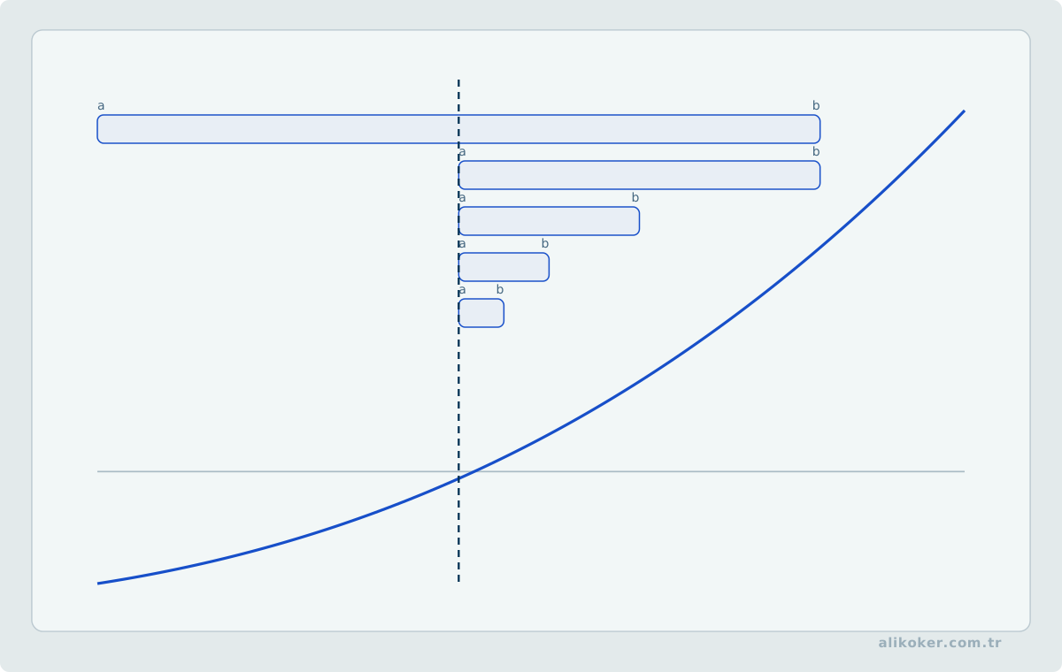
If f is continuous on [a,b] and

f(a)f(b) < 0,

then at least one root lies inside. Bisection repeatedly halves the interval and retains the half with the sign change.

After n steps the interval width is reduced by 2^n, so an explicit upper bound on the number of steps needed for a target interval tolerance can be computed from the initial bracket.

A standard sign-change bisection test generally does not detect an even-multiplicity root where the function only touches the axis without changing sign.

Stopping iterations

Possible stopping rules include interval width, successive-iterate change, residual magnitude |f(x)|, or a combination. The criterion should reflect the required accuracy and the scaling of the problem.

Regula falsi

False position also preserves a sign-changing bracket but uses the secant line through the bracket endpoints to propose the next point. It can outperform bisection on some functions, although one endpoint may remain fixed for many iterations.

Fixed-point iteration

Rewrite the equation as

x = g(x)

and iterate

x_(k+1) = g(x_k).

Local convergence is related to the behavior of g' near the fixed point; a convenient sufficient condition is |g'(x)| < 1 on an appropriate neighborhood.

Newton-Raphson method

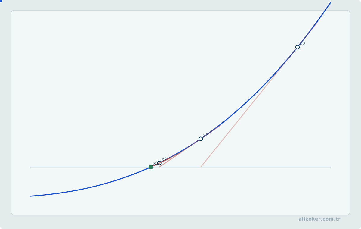
Newton's method uses the tangent line:

x_(k+1) = x_k - f(x_k)/f'(x_k).

Near a simple root and under appropriate smoothness and derivative conditions, convergence is locally quadratic. A poor initial guess or a derivative near zero can produce large steps, loss of stability, or failure to converge.

Secant method

The secant method approximates the derivative with the slope through the two most recent points:

x_(k+1) = x_k - f(x_k)(x_k-x_(k-1)) / [f(x_k)-f(x_(k-1))].

It avoids explicit derivative evaluation. It is an open method and, although it can converge rapidly from suitable starting points, it has no general convergence guarantee.

Müller method

Müller's method fits a quadratic through three recent points and uses a root of that quadratic as the next approximation. It can naturally produce complex iterates and is useful in polynomial and complex-root searches, but it does not guarantee that all roots will be found.

Comparing methods

No single method dominates every problem. Bisection emphasizes robustness under its bracketing assumptions. Newton emphasizes fast local convergence when a reliable derivative and suitable initial estimate are available. Secant avoids derivatives. Regula falsi keeps a bracket. Müller uses quadratic interpolation and can enter the complex plane.

Conditioning and algorithmic stability are different questions

Conditioning describes the problem: how much the exact mathematical answer changes when the input is perturbed. Stability describes the algorithm: how much extra error the computational procedure introduces.

A stable algorithm cannot repair an inherently ill-conditioned problem, and a well-conditioned problem can still be solved poorly by an unstable algorithm.

This distinction should be checked before interpreting a small residual as proof of an accurate solution.

Richardson extrapolation and Romberg integration

If a numerical approximation has a known leading error term, two step sizes can be combined to cancel part of that error. Richardson extrapolation uses this idea generically.

Romberg integration applies repeated Richardson extrapolation to trapezoidal-rule estimates with successively halved step sizes. It can converge quickly for sufficiently smooth integrands, but discontinuities, endpoint singularities, and highly oscillatory functions require a different strategy.

Unit 5: Interpolation

Problem

Given data

(x0,y0), (x1,y1), ..., (xn,yn),

interpolation constructs a function that passes through the supplied data points. Polynomial interpolation is a classical approach.

Simple interpolation

For two points, linear interpolation uses the straight line joining them. It is local and inexpensive but cannot represent curvature between widely separated points.

Lagrange interpolation

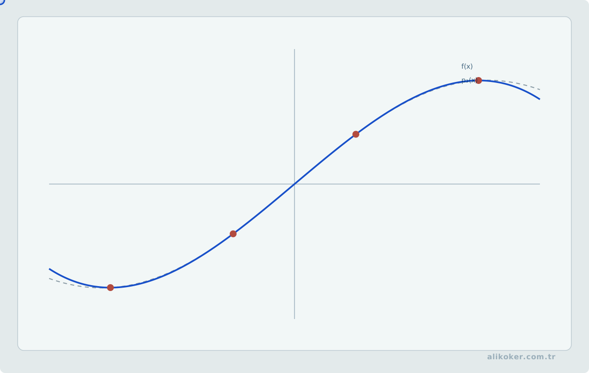
The Lagrange polynomial is

P_n(x) = Σ_i y_i L_i(x),

where

L_i(x) = Π_(j≠i) (x-x_j)/(x_i-x_j).

It gives the unique polynomial of degree at most n through n+1 distinct nodes.

Newton interpolation polynomial

Newton's divided-difference form writes the same interpolating polynomial incrementally:

P_n(x) = f[x0]
       + f[x0,x1](x-x0)
       + ...

Its structure is convenient when new nodes are added because previous coefficients need not all be discarded.

Danger of high degree

Increasing polynomial degree does not guarantee increasing accuracy. With some node distributions, high-degree interpolation can oscillate strongly, especially near interval endpoints. This is the classical Runge phenomenon.

Interpolation versus curve fitting

Interpolation forces the model through every supplied point. Curve fitting or regression instead estimates a lower-dimensional relationship and need not pass exactly through noisy observations. Extrapolation evaluates outside the data range and is generally more risky because it depends more strongly on assumptions about behavior beyond the observed interval.

Unit 6: Numerical Differentiation and Integration

When an analytical derivative or integral is unavailable, sampled function values can be used to construct numerical approximations. Truncation error and floating-point roundoff must be considered together.

Finite-difference derivatives

The forward difference is:

f'(x) ≈ [f(x+h) - f(x)] / h

and the central difference is:

f'(x) ≈ [f(x+h) - f(x-h)] / (2h)

For sufficiently smooth functions, the central formula has a higher-order truncation error for the same step size.

Making h indefinitely smaller does not indefinitely improve the answer. When h is too small, subtracting nearly equal values amplifies cancellation and roundoff. A useful step lies in the region where truncation and floating-point error are balanced.

Trapezoidal and Simpson rules

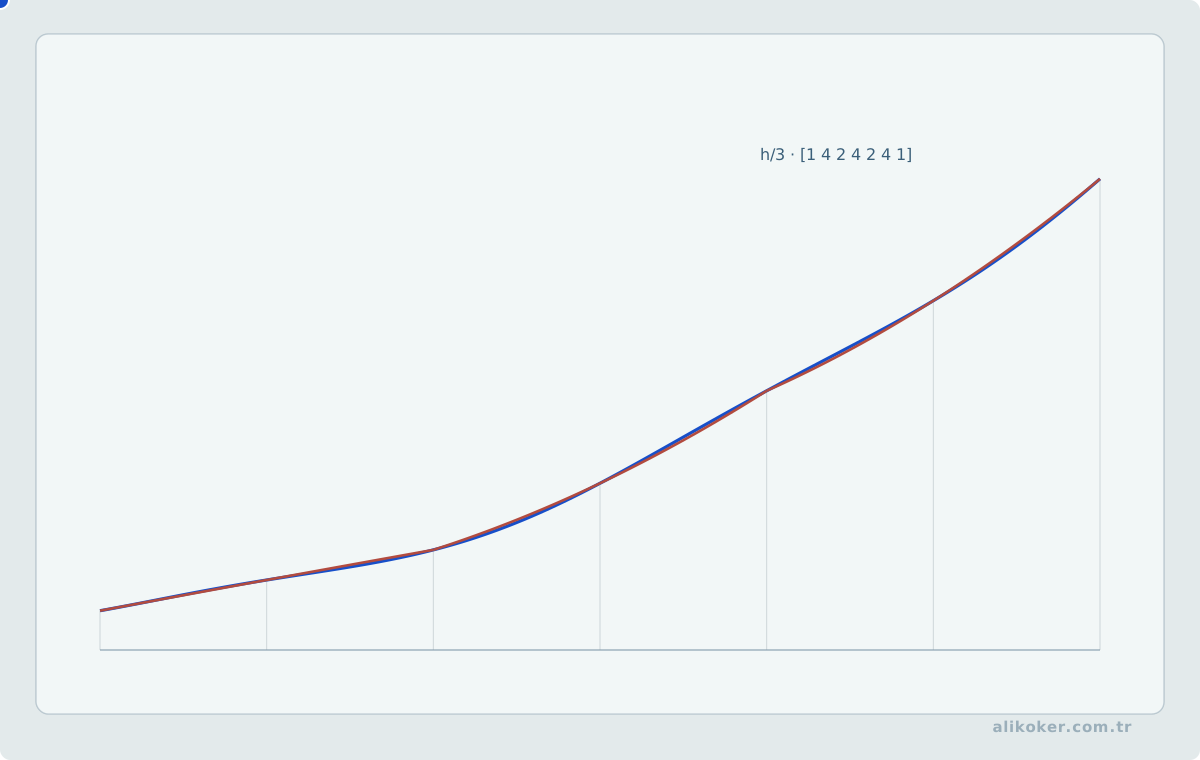
For an integral over [a,b], the trapezoidal rule approximates the function by a line:

∫ f(x) dx ≈ (b-a) [f(a)+f(b)] / 2

The composite rule applies the same idea over subintervals.

Simpson's rule uses a quadratic approximation and can provide higher accuracy for sufficiently smooth functions. Higher formal order is not automatically better for every dataset; smoothness and sampling geometry must satisfy the assumptions of the method.

Gaussian quadrature

Rather than evaluating at equally spaced points, Gaussian quadrature chooses specific nodes and weights so that a high polynomial degree can be integrated exactly with relatively few function evaluations.

The engineering choice is therefore not only "which formula has higher order?" Function-evaluation cost, singularities, fixed sample locations, and the required error bound all matter.

Unit 7: Initial-Value Problems

An initial-value problem has the form:

y' = f(t, y)
y(t0) = y0

When no analytical solution is available, time is discretized and an approximate state is advanced step by step.

Euler's method

The simplest explicit method is:

y_(n+1) = y_n + h f(t_n, y_n)

It advances along the local tangent. Euler's method is valuable pedagogically, but error may accumulate rapidly. Reducing the step generally improves accuracy while increasing computational cost.

Heun and Runge-Kutta methods

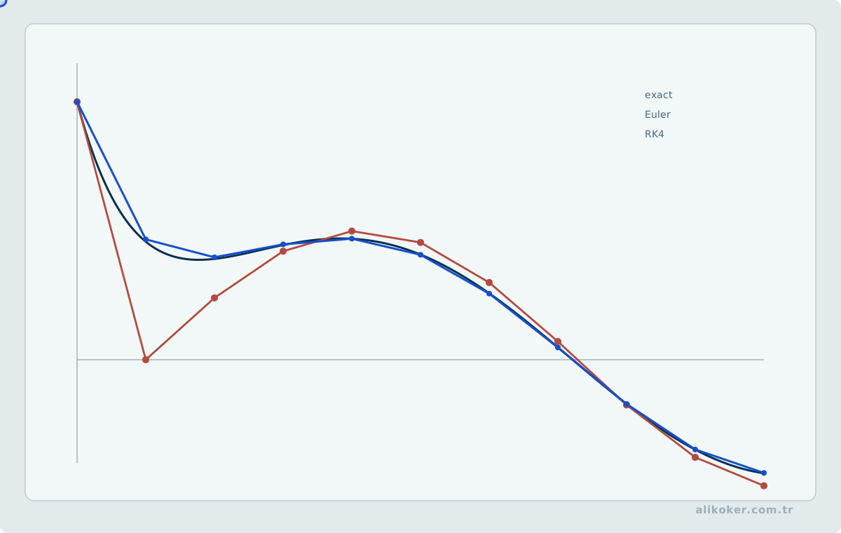
Heun's method combines the slope at the beginning of the interval with a predicted slope near its end. Classical fourth-order Runge-Kutta (RK4) evaluates four slopes:

k1 = f(tn, yn)
k2 = f(tn+h/2, yn+h k1/2)
k3 = f(tn+h/2, yn+h k2/2)
k4 = f(tn+h, yn+h k3)

and updates:

y_(n+1) = y_n + h(k1 + 2k2 + 2k3 + k4)/6

Stability and stiff systems

A numerical method can make an analytically stable system appear unstable when the step size is inappropriate. Formal order of accuracy and numerical stability are therefore separate properties.

Stiff systems may force explicit methods to use very small steps. Implicit methods can be more appropriate even though each step is computationally more expensive.

A reliable numerical ODE workflow should:

1. reduce the step and check convergence,
2. verify physical or mathematical invariants,
3. compare with another method when practical,
4. report tolerances and failure criteria explicitly.

Adaptive step size and local versus global error

For an ODE solver, local truncation error describes the error introduced by one idealized step starting from the exact state. Global error is the accumulated difference after many steps.

Adaptive methods estimate local error by comparing two approximations of different orders or step sizes. The step is accepted, rejected, enlarged, or reduced according to a tolerance contract.

A smaller step is not automatically better without limit. It increases the number of operations and can amplify roundoff, while stiff systems may require methods with a different stability region rather than simply a smaller explicit step.

General Conceptual Framework

Numerical work can be organized around a few recurring questions:

Mathematical problem
      ↓
Approximation or factorization
      ↓
Algorithm
      ↓
Finite-precision computation
      ↓
Error / residual / convergence check
      ↓
Interpretation of the numerical result

An algebraically valid formula is not automatically a good numerical algorithm. Cost, conditioning, stability, stopping criteria, and problem structure all matter.

Direct and iterative linear solvers address different computational settings. Root-finding methods trade robustness, derivative requirements, bracketing, and local speed. Interpolation reproduces data points but does not automatically provide a reliable model outside their range.

Conceptual Distinctions

Truncation error ≠ rounding error. Truncation replaces an exact process with a finite approximation; rounding arises from finite-precision arithmetic.

True error ≠ approximate iterative error. The exact error requires the exact value; successive-iterate differences are only an observable estimate.

Linear-system solution ≠ explicit matrix inversion. Forming the inverse is usually unnecessary. Direct solution with suitable pivoting or factorization is commonly cheaper and numerically preferable.

LU ≠ Cholesky. LU is a general triangular factorization under suitable conditions; Cholesky specifically exploits symmetric positive-definite structure.

Jacobi ≠ Gauss-Seidel. Jacobi uses only the previous iterate; Gauss-Seidel immediately reuses updated components.

Bracketing method ≠ unconditional guarantee. Bisection and false position rely on continuity and a valid sign-changing bracket. Under these conditions the bracket provides controlled convergence.

Bisection gives an a priori step bound. The initial interval and target tolerance provide a direct upper bound on the number of halvings required.

Newton-Raphson is locally fast, not globally guaranteed. Near a simple root under appropriate conditions it is quadratically convergent; poor starting values or small derivatives can cause large steps or failure.

Interpolation ≠ extrapolation. Extrapolation leaves the observed interval and is generally more assumption-sensitive.

Choosing a numerical method is a concrete engineering trade-off among accuracy, cost, and stability. More iterations do not automatically produce a better answer; on an ill-conditioned problem or with an unstable method, a larger computational budget can simply produce the wrong result more expensively.

Error budgets from models to floating point

Numerical error has several sources: modeling assumptions, measurement uncertainty, discretization, incomplete iteration, and floating-point rounding.

Using double does not automatically make a computation accurate. Conditioning comes first, algorithmic stability second, and representation precision after that.

Stopping criteria should combine absolute and relative tolerances with residual checks. A small change between iterations does not always mean the underlying equation is well satisfied.

Building an error budget for numerical results

Numerical discrepancy is not caused only by rounding. Modeling error, input uncertainty, discretization, iteration tolerance, and floating-point representation are distinct sources. Increasing precision may not help if another source dominates.

In a convergence study, refining the step or mesh should produce the expected order of convergence. If it does not, investigate implementation errors, boundary conditions, or violated method assumptions.

When no reference solution exists, residuals, conserved quantities, and an independent second method provide useful cross-checks. Running the same code with two parameter values is not an independent validation.

The Role of Numerical Analysis in AI Computation

AI models may be defined over real numbers, but computers execute finite-precision arithmetic and approximate algorithms. Numerical analysis therefore remains directly relevant. Larger models do not remove numerical error; they can amplify its visibility through long reduction chains and wide dynamic ranges.

Floating point and accumulated error

Simple decimal values may not be represented exactly in binary floating point. Small rounding errors can accumulate across millions of operations or become amplified by ill-conditioned computations. Matrix products, reductions, and normalizations in training and inference are all affected by data type and operation order.

FP16, BF16, and integer quantization can improve performance, but reduce precision. Mixed-precision execution is a modern form of classical error management: some operations use narrow formats while critical accumulations use wider ones.

Conditioning and stability

An ill-conditioned problem can turn small input perturbations into large output changes. A stable algorithm cannot remove that inherent sensitivity. Conversely, a well-conditioned problem can still be solved poorly by an unstable algorithm.

For least squares, forming normal equations:

(A^T A)x = A^T b

can square the condition number. QR or SVD methods can be safer. Even elementary linear regression therefore has a numerical-method dimension.

Optimization is a numerical iteration

Training commonly has the form:

θ_(k+1) = θ_k + Δθ_k

Step size, stopping criteria, gradient scale, and tolerances affect the result. Overflow, underflow, or unstable updates can occur even while the high-level model is correctly specified.

Stable evaluation of nonlinear expressions

Products of small probabilities can underflow, motivating log-likelihood:

log Π p_i = Σ log p_i

Softmax can overflow if exponentials are evaluated directly. Subtracting the maximum leaves the mathematical result unchanged while improving numerical stability:

softmax(z_i) = exp(z_i-m) / Σ exp(z_j-m)

with m=max(z).

Approximation beyond floating point

Approximate nearest-neighbor search, low-rank approximation, quantization, and pruning intentionally trade accuracy for lower cost. “Approximate” should therefore be quantified with recall, error norms, task metrics, and latency rather than treated as a qualitative label.

Parallel reductions also affect reproducibility because floating-point addition is not associative at the bit level:

(a+b)+c ≠ a+(b+c)

Small differences across hardware or execution order are not automatically defects; acceptable tolerance must be defined by the task.

Numerical analysis does not decide what an AI model should learn. It decides how reliably the intended computation survives finite precision, approximation, and iteration.

Choose the numerical method before trusting the number

Producing a number is not the same as producing a reliable approximation. Error can originate in the data or model, in truncation introduced by the method, and in rounding caused by finite-precision arithmetic. Separating these sources helps explain why a result changes.

Bisection and Newton's method illustrate different guarantees. Bisection narrows a sign-changing interval slowly but predictably when the continuity assumptions hold. Newton's method can converge very rapidly near a suitable solution, yet it can fail when the derivative is small, the initial point is poor, or the function geometry is unfavourable.

Conditioning belongs to the problem; stability belongs to the algorithm. A well-conditioned problem can be damaged by an unstable method. In an ill-conditioned problem, small perturbations in the input can create large output changes even when the numerical algorithm is implemented correctly.

Interpolation and regression also answer different questions. Interpolation constructs a function that passes through the supplied points; regression can model an underlying trend in noisy data. A high-degree polynomial passing through every sample does not guarantee reliable behaviour between samples.

For iterative methods, iteration count alone is a weak stopping criterion. Step size, residual, and the scale of the problem should be considered together. A small |x_(k+1)-x_k| does not necessarily mean that the governing equation is well satisfied. The stopping rule should be tied to the mathematical quantity the method is intended to approximate.

References

• Ahmet Yesevi Üniversitesi Bilgisayar Mühendisliği Bölümü. Sayısal Çözümleme (TBIL301) ders materyalleri.

• Gene H. Golub, Charles F. Van Loan. Matrix Computations, 4th Edition. Johns Hopkins University Press, 2013.

• Lloyd N. Trefethen, David Bau III. Numerical Linear Algebra. SIAM, 1997.

• Nicholas J. Higham. Accuracy and Stability of Numerical Algorithms, 2nd ed. SIAM, 2002.

• Nicholas J. Higham. Accuracy and Stability of Numerical Algorithms, 2nd Edition. SIAM, 2002.

• Paulius Micikevicius et al. “Mixed Precision Training.” International Conference on Learning Representations, 2018.

• Richard L. Burden, J. Douglas Faires, Annette M. Burden. Numerical Analysis, 10th Edition. Cengage, 2015.

• Steven C. Chapra, Raymond P. Canale. Numerical Methods for Engineers, 7th Edition. McGraw-Hill, 2015.

• William H. Press, Saul A. Teukolsky, William T. Vetterling, Brian P. Flannery. Numerical Recipes: The Art of Scientific Computing, 3rd Edition. Cambridge University Press, 2007.