Differential Equations: First- and Second-Order Equations

I prepared my differential-equations notes during undergraduate Computer Engineering courses in the 2013-2014 period. This revision preserves the original progression through first- and second-order differential equations while making the conditions for existence, uniqueness, and the applicability of solution methods more explicit. Later sources were used to review terminology and technical details without changing the historical course structure.

Unit 1: Fundamental Concepts and Definitions

Definition of a differential equation

A differential equation relates an unknown function to one or more of its derivatives. In an ordinary differential equation, the unknown function depends on a single independent variable. A basic first-order example is

dy/dx = f(x,y)

while a second-order equation may contain y'', y', and y together.

Classification

Differential equations are commonly classified by the number of independent variables, order, degree when defined, linearity, and whether the equation is homogeneous. This note concentrates on ordinary differential equations.

A linear equation has the unknown function and its derivatives only to the first power and does not multiply them together. Nonlinear equations do not satisfy that structure.

Order and degree

The order is the order of the highest derivative occurring in the equation. The degree is the algebraic degree of the highest-order derivative after the equation has been written as a polynomial in the derivatives; it is not defined for every differential equation.

Forms of representation

A first-order equation can be written in forms such as

y' = f(x,y)

or

M(x,y) dx + N(x,y) dy = 0.

The form often determines which solution method is convenient.

Types of solutions

A general solution contains the number of arbitrary constants expected from the order of the equation. A particular solution results after those constants are fixed by additional conditions. A singular solution, when it exists, may not be obtained from the general family by choosing constant values.

Initial-value problem

An initial-value problem specifies the value of the unknown function and, for higher-order equations, enough derivatives at one point. For example,

y' = f(x,y),   y(x0) = y0

combines a differential equation with one initial condition.

Boundary-value problem

A boundary-value problem gives conditions at different points. A second-order equation may, for example, specify y(a) and y(b). Unlike a standard initial-value problem, a boundary-value problem may have no solution, one solution, or multiple solutions.

Existence and uniqueness

The fact that an equation is written down does not by itself guarantee a unique solution. For a first-order initial-value problem, continuity of f helps establish local existence, while suitable regularity with respect to y provides a standard route to uniqueness. The exact hypotheses matter.

Modeling physical phenomena

Differential equations model change. Population growth, radioactive decay, heat transfer, mechanical vibration, electrical circuits, and control systems can all be described by relations between state variables and their rates of change. The mathematical equation is a model, so the assumptions behind it remain part of the engineering problem.

Unit 2: Classification of First-Order Equations

Forms of representation

Before applying a method, the equation should be rewritten into a form that exposes its structure. Typical patterns are separable, exact, homogeneous, linear, and Bernoulli equations.

Classification

A first-order equation may satisfy more than one recognizable pattern. Classification is therefore not only a naming exercise; it is a way of selecting an efficient transformation or integration method.

Unit 3: Separable Equations

General solution

An equation of the form

dy/dx = g(x) h(y)

is separable when it can be rearranged as

dy / h(y) = g(x) dx.

Integrating both sides gives the implicit or explicit general solution.

Points to check in practice

Division by a function of y can discard solutions at points where that function is zero. Constant solutions should therefore be checked before division. Domains and integration constants must also be handled consistently.

Application areas

Separable models arise in elementary growth and decay, simple cooling models, some motion equations, and other systems where the state and independent variable factors can be isolated.

Unit 4: Exact Differential Equations

Exact differential

For a differentiable function F(x,y),

dF = Fx dx + Fy dy.

This gives the basis for identifying an equation as the differential of a potential function.

Exact differential equation

An equation

M(x,y) dx + N(x,y) dy = 0

is exact on a suitable domain if there is a function F such that

Fx = M,   Fy = N.

Its solution is then

F(x,y) = C.

Exactness criterion

Under the usual differentiability assumptions, exactness is tested locally by

∂M/∂y = ∂N/∂x.

Domain conditions should not be ignored when a global conclusion is required.

Finding the general solution

Integrate M with respect to x or N with respect to y, retain the unknown function of the other variable, and determine that function by differentiating and comparing with the remaining coefficient.

Integrating factor

A non-exact equation can sometimes be multiplied by a function μ so that

μM dx + μN dy = 0

becomes exact. An integrating factor is not arbitrary; its useful form depends on the structure of the equation.

Unit 5: Homogeneous Differential Equations

Homogeneous function

A function is homogeneous of degree k if

f(tx,ty) = t^k f(x,y).

Homogeneous differential equation

For a first-order homogeneous equation, the right-hand side can often be expressed as a function of the ratio y/x or x/y.

Solution method

With the substitution

y = vx

we have

dy/dx = v + x dv/dx.

The resulting equation is commonly separable in v and x. After integration, substitute v = y/x back into the result.

Equations reducible to homogeneous form

Translations of the variables can sometimes eliminate constant terms and convert an equation into homogeneous form. The transformation should be chosen from the algebraic structure rather than applied mechanically.

Unit 6: First-Order Linear Equations

Definition

The standard form is

y' + P(x)y = Q(x).

When A(x) and B(x) in an equivalent representation satisfy suitable regularity conditions, the integrating-factor method gives a systematic general solution.

Method 1: variation of the constant

First solve the homogeneous equation

y' + P(x)y = 0.

Instead of treating the integration constant as fixed, replace it by a function and determine that function from the nonhomogeneous equation.

Method 2: general solution formula

Using the integrating factor

μ(x) = exp(∫P(x) dx),

the equation becomes

(μy)' = μQ.

Therefore

y = [∫ μ(x)Q(x) dx + C] / μ(x).

Method 3: integrating factor

The integrating-factor derivation is often the most direct because it turns the left-hand side into a product derivative. The formula is meaningful on intervals where the coefficient functions satisfy the required conditions.

Bernoulli equation

A Bernoulli equation has the form

y' + P(x)y = Q(x)y^n.

For n ≠ 0,1, the substitution

z = y^(1-n)

reduces it to a first-order linear equation.

Mechanical application

First-order linear equations occur when a force or response is proportional to a state variable or its first derivative. The differential equation describes the dynamic law, while initial conditions select the physical trajectory.

Unit 7: Second-Order Linear Homogeneous Equations with Constant Coefficients

Definition

The standard equation is

ay'' + by' + cy = 0,   a ≠ 0.

Structure of the solutions

Because the equation is linear and homogeneous, linear combinations of independent solutions are again solutions. A second-order equation requires two linearly independent solutions for its general solution.

Characteristic equation

Assuming y = e^(rx) gives

ar^2 + br + c = 0.

The roots determine the solution form:

• two distinct real roots: C1 e^(r1 x) + C2 e^(r2 x),
• one repeated real root: (C1 + C2 x)e^(rx),
• complex roots α ± iβ: e^(αx)[C1 cos(βx) + C2 sin(βx)].

Mechanical vibrations

The mass-spring-damper model leads to

m x'' + c x' + kx = 0.

The characteristic roots distinguish underdamped, critically damped, and overdamped behavior.

Simple harmonic motion

When damping is absent,

m x'' + kx = 0

has sinusoidal solutions. The natural angular frequency is

ωn = sqrt(k/m).

Damped vibration

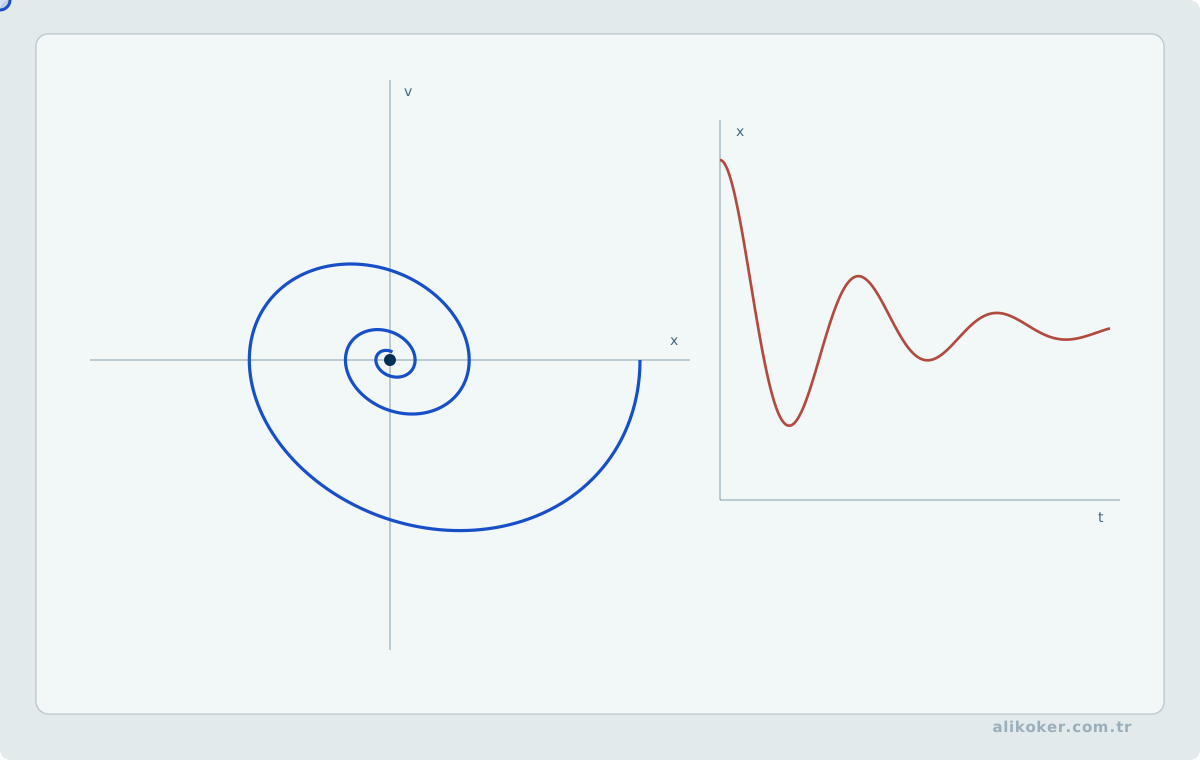
Damping modifies the amplitude envelope and may also modify the observed oscillation frequency. The discriminant of the characteristic equation gives the basic classification.

Unit 8: Second-Order Linear Nonhomogeneous Equations with Constant Coefficients

Structure of the general solution

For

ay'' + by' + cy = f(x),

the solution is

y = yh + yp,

where yh solves the homogeneous equation and yp is any particular solution.

Variation of parameters

Variation of parameters constructs a particular solution from two independent homogeneous solutions. It is general but usually requires integration.

Method of undetermined coefficients

When f(x) belongs to a suitable family such as polynomials, exponentials, sines, cosines, or finite combinations of them, a trial function with unknown coefficients can be substituted into the equation.

Resonance

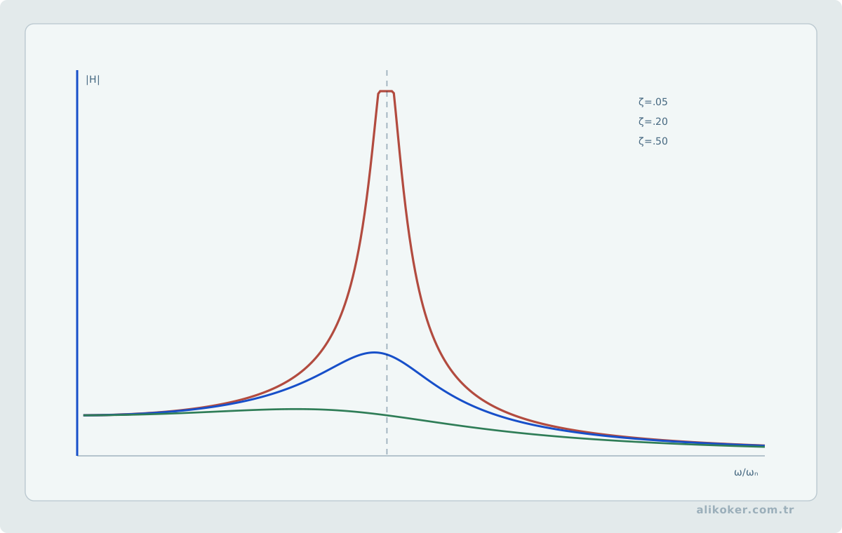
If the trial form overlaps with a homogeneous solution, it must be multiplied by a sufficient power of x. In vibration models, forcing near a natural frequency can produce resonance behavior; damping changes the physical response.

Comparing the methods

Undetermined coefficients is efficient for restricted forcing functions. Variation of parameters is more general. Method selection should follow the form of the forcing term and the desired representation of the solution.

Unit 9: Operator Method

Differential operator

Let

D = d/dx.

Then a constant-coefficient equation can be written as

P(D)y = f(x).

This notation exposes the polynomial structure of the differential operator.

Finding a particular solution with operators

Formally,

yp = 1/P(D) f(x).

The expression is interpreted through algebraic operator rules that depend on the forcing function; it is not ordinary scalar division.

Polynomial forcing

For a polynomial f(x), expansions of the inverse operator can terminate after finitely many differentiations because higher derivatives vanish.

Exponential forcing

For

f(x) = e^(ax),

the shift property leads to evaluation involving P(a) when P(a) ≠ 0. If P(a) = 0, the overlapping homogeneous factor must be handled separately.

Sine or cosine forcing

Trigonometric forcing can be handled by using the relation between repeated derivatives and the operator polynomial, or by representing sine and cosine through complex exponentials.

Exponential times another function

For e^(ax)v(x), the shift rule effectively replaces D by D+a in the operator acting on v.

Sum of different forcing types

Linearity allows the particular solution for a sum of forcing terms to be formed by adding particular solutions for the individual terms.

Place of the method

Operator notation is compact for constant-coefficient linear equations, but it does not replace the conceptual distinction between homogeneous and particular solutions or the conditions behind each algebraic shortcut.

General Conceptual Framework

The course can be read as a sequence of structural questions:

What type of equation is this?
        ↓
Can it be separated, made exact, or reduced by substitution?
        ↓
If it is linear, what does its homogeneous part imply?
        ↓
Which initial or boundary conditions select the required solution?
        ↓
What assumptions make existence and uniqueness valid?

First-order equations emphasize classification and transformations. Second-order constant-coefficient equations connect algebraic roots with dynamic behavior. Initial conditions determine a trajectory; boundary conditions impose constraints at different points. A solution method is valid because the equation has a certain structure, not because a formula is memorized.

Conceptual Distinctions

Order ≠ degree. Order is determined by the highest derivative; degree is an algebraic property that is defined only when the equation is polynomial in its derivatives.

General solution ≠ particular solution. A general solution contains arbitrary constants; a particular solution satisfies specified conditions or corresponds to fixed constants.

Initial-value problem ≠ boundary-value problem. Initial conditions are imposed at one point, whereas boundary conditions can be imposed at different points.

Existence ≠ uniqueness. A solution may exist without being unique. Standard theorems require explicit hypotheses.

Exact equation ≠ arbitrary differential form. Exactness means that the coefficients are partial derivatives of a common potential function on the relevant domain.

Homogeneous first-order equation ≠ homogeneous linear equation. The word homogeneous refers to different structural properties in these two contexts.

Complementary solution ≠ particular solution. For a linear nonhomogeneous equation, the complete solution is the sum of a homogeneous solution and one particular solution.

Characteristic roots ≠ initial conditions. Characteristic roots determine the form of the homogeneous solution; initial conditions determine the constants.

Undetermined coefficients ≠ variation of parameters. The first is efficient for restricted forcing families; the second is more general.

An initial-value problem is not automatically unique. Existence and uniqueness depend on appropriate hypotheses. A boundary-value problem can have no solution, one solution, or several solutions.

References

• Ahmet Yesevi Üniversitesi Bilgisayar Mühendisliği Bölümü. Diferansiyel Denklemler (TBIL204) ders materyalleri.
• William E. Boyce, Richard C. DiPrima, Douglas B. Meade. Elementary Differential Equations and Boundary Value Problems, 11th Edition. Wiley, 2017.
• Dennis G. Zill. A First Course in Differential Equations with Modeling Applications, 11th Edition. Cengage, 2018.
• Morris Tenenbaum, Harry Pollard. Ordinary Differential Equations. Dover, 1985.
• George F. Simmons. Differential Equations with Applications and Historical Notes, 3rd Edition. CRC Press, 2016.
• Ernst Hairer, Syvert P. Nørsett, Gerhard Wanner. Solving Ordinary Differential Equations I: Nonstiff Problems, 2nd Revised Edition. Springer, 1993.