Linear Algebra: Matrices, Linear Systems and Eigenvalues

I prepared my linear-algebra notes during undergraduate Computer Engineering courses in the 2013-2014 period. This revision preserves the original sequence from linear systems and matrices through determinants, vectors, rank, eigenvalues, and diagonalization, while reviewing numerical and conceptual distinctions with later sources.

Unit 1: Linear Equations and Matrices

Linear equation

A linear equation in variables x1, x2, ..., xn has the form

a1 x1 + a2 x2 + ... + an xn = b.

The coefficients and constant term are scalars. Variables appear only to the first power and are not multiplied together.

System of linear equations

A linear system is a collection of linear equations sharing the same unknowns. Depending on consistency and rank, a system can have one solution, no solution, or infinitely many solutions.

Geometry of a two-variable system

In two dimensions, each nondegenerate linear equation represents a line. Two distinct nonparallel lines intersect at one point; parallel distinct lines have no common solution; coincident lines represent infinitely many common solutions.

Elementary operations and elimination

The solution set is preserved by exchanging equations, multiplying an equation by a nonzero scalar, and adding a multiple of one equation to another. These are the algebraic basis of elimination.

Matrix concept

A matrix organizes coefficients in rows and columns. An m x n matrix has m rows and n columns. Matrices provide a compact representation of systems and linear transformations.

Addition, subtraction, and scalar multiplication

Matrices of the same dimensions are added or subtracted element by element. Scalar multiplication multiplies every entry by the same scalar.

Matrix multiplication

If A is m x n and B is n x p, then

(AB)_ij = Σ_k a_ik b_kj.

The product exists only when the inner dimensions match. In general,

AB ≠ BA.

Special matrices

Frequently used forms include the zero matrix, identity matrix, diagonal matrix, scalar matrix, upper and lower triangular matrices, symmetric matrix, and transpose. Structural properties can simplify later computations.

Unit 2: Solving Linear Systems with Matrices

Matrix representation

A linear system can be written as

Ax = b.

Here A is the coefficient matrix, x is the unknown vector, and b is the right-hand-side vector.

Augmented matrix

The augmented matrix

[A | b]

stores the coefficients and right-hand side in one array and is convenient for row reduction.

Gaussian elimination

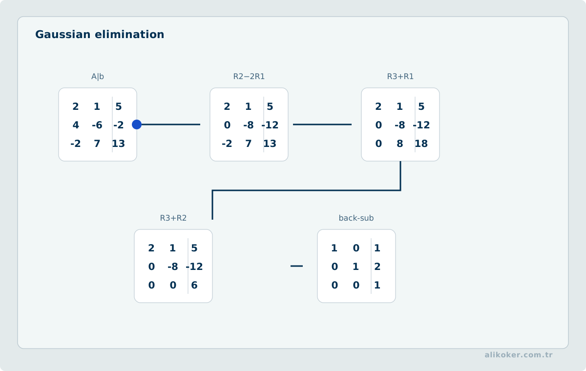
Gaussian elimination uses elementary row operations to transform the augmented matrix to row-echelon or upper-triangular form. Back substitution then recovers the unknowns.

Gauss-Jordan method

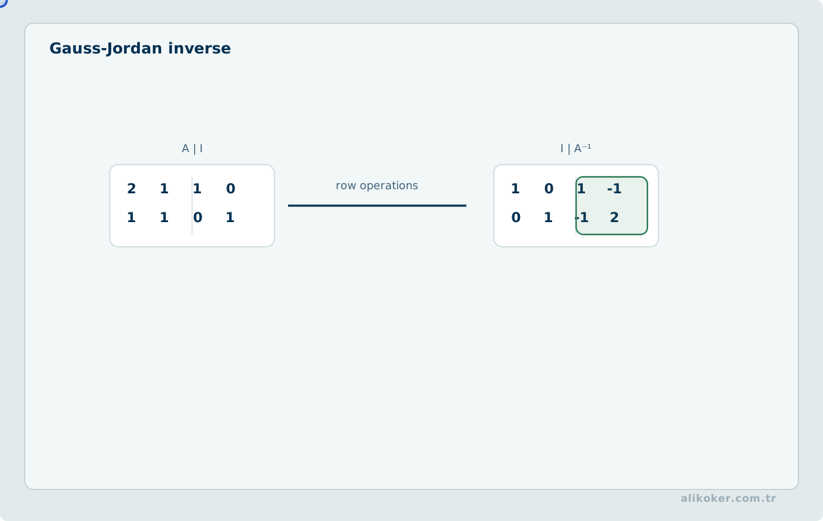
Gauss-Jordan elimination continues row reduction until pivot columns are reduced further, ideally producing reduced row-echelon form. This makes free variables and consistency conditions directly visible.

Reading the solution set

A contradictory row such as

0 0 ... 0 | c,   c ≠ 0

shows inconsistency. If the system is consistent and every variable column contains a pivot, the solution is unique. Free variables imply infinitely many solutions.

Inverse matrix

For a square matrix A, an inverse A^-1 satisfies

AA^-1 = A^-1A = I.

An inverse exists exactly when A is nonsingular.

Solving with the inverse matrix

If A is invertible,

Ax = b
x = A^-1 b.

This identity is useful conceptually. In practical numerical computation, explicit inversion is usually not the preferred way to solve a single linear system; factorization or elimination is more efficient.

Unit 3: Determinants

Definition of the determinant

The determinant maps a square matrix to a scalar. It captures information about invertibility, orientation, and volume scaling.

Second- and third-order determinants

For

A = [a b; c d],

det(A) = ad - bc.

For 3 x 3 matrices, cofactor expansion or Sarrus' rule can be used. Sarrus' rule applies only to 3 x 3 determinants and does not generalize to higher dimensions.

Properties of determinants

Important properties include:

• interchanging two rows changes the sign;
• multiplying a row by k multiplies the determinant by k;
• adding a multiple of one row to another leaves the determinant unchanged;
• a triangular matrix has determinant equal to the product of its diagonal entries;
• det(AB) = det(A)det(B);
• det(A^T) = det(A).

Determinants using row operations

Row reduction can transform the matrix to triangular form while tracking row exchanges and scalings. This avoids the combinatorial cost of a large cofactor expansion.

Minor and cofactor

The minor M_ij is the determinant obtained after deleting row i and column j. The cofactor is

C_ij = (-1)^(i+j) M_ij.

Cofactor expansion

A determinant can be expanded along any row or column:

det(A) = Σ_j a_ij C_ij.

The value is independent of the chosen expansion row or column.

Unit 4: Invertibility, Adjugate Matrix, and Cramer's Rule

Invertibility criterion using the determinant

For a square matrix,

det(A) ≠ 0

is equivalent to invertibility. A zero determinant means the matrix is singular.

Adjugate matrix

The adjugate is the transpose of the cofactor matrix. For a nonsingular matrix,

A^-1 = adj(A) / det(A).

This is a closed general formula and is useful for theory and small matrices. For large numerical problems, cofactor-based inversion is normally replaced by factorization and linear-system solvers.

Cramer's rule

For a nonsingular square system,

x_i = det(A_i)/det(A),

where A_i is obtained by replacing column i of A with b. The rule is mathematically elegant but not computationally efficient for large systems.

Unit 5: Vectors

Scalar and vector quantities

A scalar has magnitude only. A vector has magnitude and direction and can be represented by ordered components in a chosen coordinate system.

Vector operations

Vectors can be added, subtracted, and multiplied by scalars componentwise. These operations satisfy the vector-space laws.

Components and magnitude

For

v = (v1, v2, ..., vn),

the Euclidean magnitude is

||v|| = sqrt(v1^2 + v2^2 + ... + vn^2).

Dot product

The dot product is

u·v = Σ_i u_i v_i.

In Euclidean space,

u·v = ||u|| ||v|| cos θ.

For nonzero vectors, a zero dot product means orthogonality.

Cross product

In three dimensions,

u x v

is perpendicular to both u and v and has magnitude

||u x v|| = ||u|| ||v|| sin θ.

If two nonzero vectors have zero cross product, they are parallel.

Scalar triple product

The scalar triple product

u · (v x w)

represents the signed volume of the parallelepiped generated by the three vectors. A zero value indicates coplanarity.

Linear combination

A vector v is a linear combination of v1,...,vk if

v = c1 v1 + ... + ck vk.

The set of all such combinations is their span.

Linear dependence and independence

Vectors are linearly independent if

c1 v1 + ... + ck vk = 0

implies all coefficients are zero. Otherwise they are linearly dependent.

Unit 6: Rank and the Structure of Solutions

Rank of a matrix

The rank is the dimension of the row space, equivalently the column space. Computationally it equals the number of pivots in a row-echelon form.

Rank and linear independence

Rank measures how many independent row or column directions the matrix contains. A set of columns is independent exactly when those columns contribute separate pivot directions.

Linear systems and rank

For

Ax = b,

the system is consistent exactly when

rank(A) = rank([A|b]).

If this common rank equals the number of unknowns, the solution is unique. If it is smaller, consistent systems have free variables and infinitely many solutions.

Homogeneous systems

For

Ax = 0,

the zero vector is always a solution. A nontrivial solution exists when the null space has positive dimension; for a square matrix this occurs when det(A)=0.

Comparing solution methods

Gaussian elimination is the general direct framework. Gauss-Jordan exposes reduced form and free variables. Inverse and Cramer formulas are useful conceptually and for small problems, but they are not preferred for large numerical systems.

Unit 7: Eigenvalues and Eigenvectors

Basic concept

A nonzero vector v is an eigenvector of A if

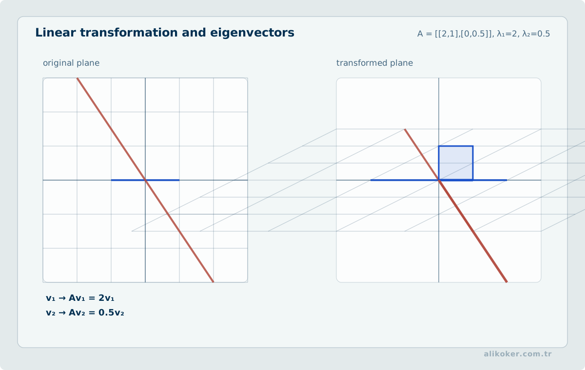
Av = λv.

The scalar λ is the corresponding eigenvalue. The transformation changes the magnitude and possibly the sign/direction along that eigenvector without changing its one-dimensional span.

Characteristic equation

Rearranging gives

(A - λI)v = 0.

A nonzero solution exists only if

det(A - λI) = 0.

This is the characteristic equation.

Computation procedure

First solve the characteristic equation for eigenvalues. For each eigenvalue, solve

(A - λI)v = 0

to obtain the corresponding eigenspace.

Properties of eigenvalues

The sum of eigenvalues counted with algebraic multiplicity equals the trace, and their product equals the determinant. For triangular matrices, the eigenvalues are the diagonal entries.

Basis and dimension

A basis is a linearly independent spanning set. Every basis of a finite-dimensional vector space contains the same number of vectors; that number is the dimension.

Diagonalization

A matrix is diagonalizable if there is an invertible matrix P such that

A = P D P^-1,

with diagonal D. The columns of P are independent eigenvectors. Having n linearly independent eigenvectors is the key requirement for an n x n matrix.

Orthogonality and orthonormality

Vectors are orthogonal when their dot product is zero. They are orthonormal when they are also unit vectors. Orthonormal bases simplify coordinates, projections, and numerical computation.

Gram-Schmidt method

Gram-Schmidt converts an independent set into an orthogonal or orthonormal set spanning the same subspace. Each new vector has its projections onto the previously constructed directions removed.

Diagonalization of symmetric matrices

A real symmetric matrix has real eigenvalues and can be diagonalized by an orthogonal matrix:

A = Q D Q^T.

This spectral structure is particularly important in numerical analysis, optimization, and quadratic forms.

General Conceptual Framework

The course connects systems, matrices, vector spaces, and transformations:

Linear equations
      ↓
Matrix representation
      ↓
Row reduction / rank
      ↓
Vector spaces and independence
      ↓
Linear transformations
      ↓
Eigenvalues and invariant directions

Determinants provide compact structural tests, but row reduction and factorization are the practical tools for systems. Rank explains consistency and degrees of freedom. Eigenvectors describe directions preserved by a linear transformation and lead to diagonal representations when enough independent eigenvectors exist.

Conceptual Distinctions

Matrix multiplication ≠ elementwise multiplication. The row-by-column rule defines the ordinary product, and multiplication is generally not commutative.

Determinant ≠ rank. The determinant is a scalar defined for square matrices; rank is defined for rectangular matrices and measures independent directions.

Sarrus' rule ≠ a general determinant algorithm. It applies only to 3 x 3 matrices.

Inverse formula ≠ preferred large-scale solver. The adjugate formula is mathematically valid, but direct factorization or elimination is usually preferable numerically.

Dot product ≠ cross product. A zero dot product indicates orthogonality. For two nonzero vectors in three dimensions, a zero cross product indicates parallelism.

Linear dependence ≠ geometric equality. Dependence means that at least one vector can be expressed from the others through a nontrivial linear relation.

**Rank(A) ≠ rank([A|b]) in an inconsistent system.** Equality is the consistency criterion.

Eigenvalue ≠ eigenvector. The eigenvalue is a scalar; the eigenvector is a nonzero direction satisfying Av=λv.

Algebraic multiplicity ≠ geometric multiplicity. Repetition in the characteristic polynomial does not automatically provide the same number of independent eigenvectors.

Diagonalizable ≠ invertible. A matrix may be diagonalizable and singular, or invertible without being diagonalizable.

Orthogonal ≠ orthonormal. Orthonormal vectors are orthogonal and also normalized to unit length.

References

• Ahmet Yesevi Üniversitesi Bilgisayar Mühendisliği Bölümü. Lineer Cebir (TBIL203) ders materyalleri.
• Gilbert Strang. Introduction to Linear Algebra, 5th Edition. Wellesley-Cambridge Press, 2016.
• Howard Anton, Chris Rorres. Elementary Linear Algebra, 12th Edition. Wiley, 2019.
• David C. Lay, Steven R. Lay, Judi J. McDonald. Linear Algebra and Its Applications, 6th Edition. Pearson, 2021.
• Gene H. Golub, Charles F. Van Loan. Matrix Computations, 4th Edition. Johns Hopkins University Press, 2013.
• Lloyd N. Trefethen, David Bau III. Numerical Linear Algebra. SIAM, 1997.
• Roger A. Horn, Charles R. Johnson. Matrix Analysis, 2nd Edition. Cambridge University Press, 2012.