Calculus II: Sequences, Series and Multivariable Analysis

The 2013-2014 Mathematics II syllabus has two clear axes: sequences and series, and multivariable analysis. Convergence conditions, multivariable derivatives and integration methods connect those axes through a common analytical language.

The two halves can appear unrelated at first. Sequences and series ask when an infinite process approaches a meaningful value, while multivariable analysis carries the same limit idea into higher-dimensional spaces. Making that common foundation explicit helps separate conceptual conditions from routine algebraic manipulation.

Unit 1: Limits of Sequences

Definition of a numerical sequence

A numerical sequence is a function whose domain is usually the positive integers:

a: N → R,   n ↦ a_n.

The index records order, so a sequence is more than a set of values.

Operations on sequences

Given sequences (a_n) and (b_n), sums, differences, products, and quotients are defined term by term wherever denominators are nonzero. Scalar multiplication is also defined termwise.

Bounded and unbounded sequences

A sequence is bounded above if there is an M with a_n ≤ M for every n, bounded below analogously, and bounded when both conditions hold. Boundedness alone does not imply convergence.

Supremum and infimum of a sequence

The set of sequence values can have a least upper bound sup a_n and greatest lower bound inf a_n. These notions summarize bounds even when the extrema are not attained by a term.

Limit of a sequence

The statement

lim_(n→∞) a_n = L

means that for every ε>0, there is an index N such that

|a_n - L| < ε

whenever n≥N.

Properties of convergent sequences

A convergent sequence has a unique limit and is bounded. Standard algebraic limit laws apply to sums, products, and quotients under the usual denominator condition.

Subsequences

A subsequence is obtained by choosing increasing indices n_k. Every subsequence of a convergent sequence converges to the same limit. Divergent sequences can nevertheless possess convergent subsequences.

Monotone sequences

A monotone increasing sequence satisfies a_(n+1) ≥ a_n; a monotone decreasing sequence satisfies the reverse inequality. A bounded monotone sequence converges.

Bolzano-Weierstrass theorem

Every bounded sequence in R^n has a convergent subsequence. In one dimension this connects boundedness with the existence of accumulation behavior even when the full sequence does not converge.

Cauchy sequences

A sequence is Cauchy if its terms eventually become arbitrarily close to one another:

for every ε>0, there is N such that
|a_n-a_m|<ε for n,m≥N.

In the real numbers, a sequence is convergent exactly when it is Cauchy. This equivalence relies on completeness.

Unit 2: Numerical Series

Definition of a series

A series

Σ_(n=1)^∞ a_n

is studied through its sequence of partial sums

S_N = Σ_(n=1)^N a_n.

The series converges if (S_N) converges.

Convergent and divergent series

If the partial sums have a finite limit, the series is convergent; otherwise it diverges. Divergence can mean growth without bound, oscillation, or failure to approach one finite value.

Necessary condition for convergence

A necessary condition is

a_n → 0.

It is not sufficient. The harmonic series is the standard counterexample.

Properties of convergent series

Finite changes to the initial terms do not affect convergence. Constant multiples and sums of convergent series remain convergent. Manipulating infinite series requires attention to convergence, especially when terms are rearranged.

Remainder of a series

For a convergent series with sum S, the remainder after N terms is

R_N = S - S_N.

Convergence tests and integral estimates can sometimes provide explicit bounds for R_N.

Cauchy criterion for series

A series converges exactly when its tails can be made arbitrarily small:

|a_(n+1)+...+a_m| < ε

for sufficiently large m>n.

Positive-term series

When every term is nonnegative, the partial sums are monotone increasing. Such a series converges exactly when its partial sums are bounded above.

Integral test

For a positive, continuous, decreasing function f with a_n=f(n), the series Σa_n and the improper integral ∫f(x)dx have the same convergence behavior. The integral can also bound the remainder.

Comparison test

If 0≤a_n≤b_n eventually and Σb_n converges, then Σa_n converges. If a_n≥b_n≥0 eventually and Σb_n diverges, then Σa_n diverges.

D'Alembert ratio test

For positive terms, if

L = lim |a_(n+1)/a_n|,

then L<1 implies absolute convergence and L>1 implies divergence. The case L=1 is inconclusive.

Cauchy root test

If

L = limsup |a_n|^(1/n),

then L<1 gives absolute convergence and L>1 divergence. Again, the boundary case requires another argument.

Raabe test

Raabe's criterion refines the ratio test for some positive series when the ordinary ratio limit approaches one. Its usefulness lies in detecting more subtle decay rates.

Alternating series

An alternating series of decreasing positive magnitudes tending to zero converges by the Leibniz criterion. The first omitted term bounds the magnitude of the remainder under these conditions.

Absolute and conditional convergence

A series converges absolutely if

Σ |a_n|

converges. Absolute convergence implies convergence. A series that converges but not absolutely is conditionally convergent.

Riemann rearrangement theorem

A conditionally convergent real series can be rearranged to change its sum or even to diverge. This is why arbitrary rearrangement is safe for absolutely convergent series but not for conditionally convergent ones.

Dirichlet and Abel tests

These tests establish convergence for products of sequences when one factor has controlled partial sums and the other has suitable monotone or bounded behavior. They are particularly useful for oscillatory series.

Power series

A power series centered at a is

Σ c_n (x-a)^n.

There is a radius R such that the series converges absolutely for |x-a|<R and diverges for |x-a|>R; endpoints must be tested separately.

Taylor and Maclaurin series

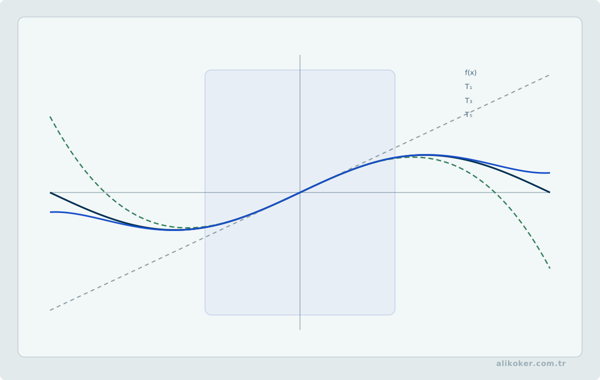
For a sufficiently regular function, Taylor's series is built from derivatives at a point:

Σ f^(n)(a)(x-a)^n/n!.

Maclaurin is the special case a=0. A formal Taylor series represents the function only where the remainder tends to zero.

Fourier series

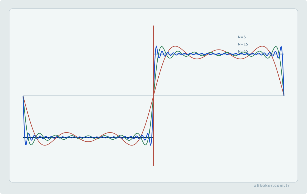
A Fourier series represents a periodic function through sine and cosine components. Coefficients are obtained from orthogonality integrals. Convergence at discontinuities requires care; pointwise behavior can differ from uniform behavior.

Absolute, conditional, and uniform convergence

For a numerical series, absolute convergence is stronger than ordinary convergence:

Σ |a_n| < ∞ => Σ a_n converges.

Conditional convergence requires more care because rearranging terms can change the sum. For sequences of functions, pointwise convergence is also weaker than uniform convergence. Uniform convergence controls the error with one bound valid over the whole domain and is important when exchanging limits with integration or differentiation.

These distinctions prevent a common mistake: treating every convergent sequence or series as if algebraic operations could be interchanged without additional hypotheses.

Unit 3: Multivariable Functions

Multivariable function and domain

A function such as

f: R^2 → R,   z=f(x,y)

assigns one value to each point in a domain of the plane. Its graph is a surface in three-dimensional space.

Limit and continuity

The limit

lim_((x,y)→(a,b)) f(x,y)=L

must be the same along every path approaching (a,b). Different path limits prove that a limit does not exist, although agreement along several paths alone does not prove existence.

Continuity requires the function value to exist and equal the limit.

Partial derivatives

Partial differentiation changes one variable while holding the others fixed:

f_x = ∂f/∂x,   f_y = ∂f/∂y.

Higher and mixed partial derivatives follow by repeated differentiation.

Differentiability and total differential

Differentiability is stronger than the mere existence of partial derivatives. Near a differentiability point,

Δf = f_x Δx + f_y Δy + o(||(Δx,Δy)||).

The linear part is the total differential.

Chain rule

If x and y depend on t,

df/dt = f_x dx/dt + f_y dy/dt.

The Jacobian generalizes this composition rule to vector-valued mappings.

Homogeneous functions and Euler's theorem

If

f(tx,ty)=t^k f(x,y),

then, under differentiability,

x f_x + y f_y = k f.

Implicit functions

An equation F(x,y)=0 can locally define one variable as a function of another under an appropriate nonzero partial-derivative condition. Implicit differentiation then gives derivative information without solving explicitly.

Jacobian

For a coordinate transformation (u,v)→(x,y), the Jacobian determinant

J = ∂(x,y)/∂(u,v)

measures local oriented area scaling. In multiple integrals its absolute value appears in change-of-variables formulas.

Coordinate transformations

Cartesian, polar, cylindrical, and spherical coordinate systems simplify problems with matching geometry. A valid transformation must include the correct domain and Jacobian factor.

Functional dependence

Functions can satisfy a relation that makes them not independent. Jacobian rank is one tool for studying local functional dependence.

Taylor formula

A multivariable Taylor expansion uses partial derivatives to approximate a function near a point. The quadratic terms involve the Hessian matrix and are central to local extremum classification.

Unconstrained extrema

At an interior differentiable local extremum,

∇f = 0

is a necessary condition. The Hessian can classify nondegenerate critical points as minima, maxima, or saddles.

Constrained extrema and Lagrange multipliers

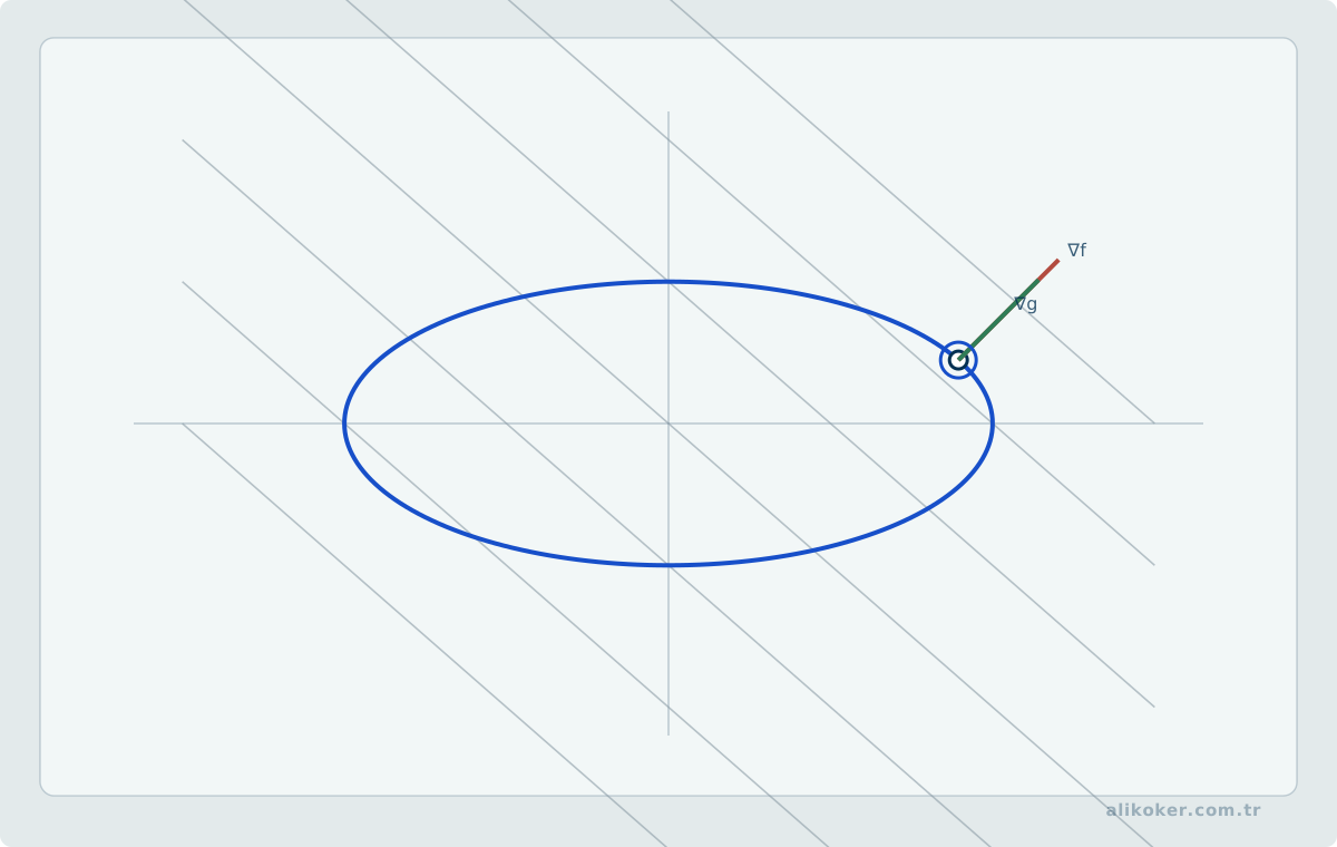
For a constraint g(x,y)=c, a regular constrained extremum satisfies

∇f = λ ∇g.

The method encodes the fact that allowable tangent directions cannot increase f to first order.

Curves, tangent vector, and normal plane

For a parametric curve r(t), the derivative r'(t) is a tangent vector when nonzero. A plane normal to the curve at a point has the tangent as its normal vector.

Surfaces, tangent plane, and normal vector

For an implicit surface F(x,y,z)=c, the gradient

∇F

is normal to the level surface where it is nonzero. The tangent plane is therefore defined from the gradient.

Gradient

∇f = (f_x,f_y,f_z)

points in the direction of steepest local increase, and its norm gives the maximum directional derivative.

Directional derivative

For a unit vector u,

D_u f = ∇f · u.

Divergence, curl, and Laplacian

For a vector field F, divergence measures local source/sink behavior and curl measures local rotation. For a scalar field,

Δf = ∇·∇f

is the Laplacian.

Change of variables and the Jacobian determinant

A multivariable substitution changes both coordinates and local area or volume. For a transformation (u,v) -> (x,y), the area element becomes

dx dy = |det J| du dv

where J is the Jacobian matrix of partial derivatives.

The determinant is a local scale factor. Omitting it produces a result in the wrong measure even when the transformed region is correct. The same principle appears in probability-density transformations, continuum mechanics, and coordinate changes used in numerical integration.

Green, Stokes, and Gauss as one structural idea

Green's theorem, Stokes' theorem, and the divergence theorem connect a derivative integrated over a region to a quantity integrated over its boundary. The dimensions and orientation differ, but the structural pattern is the same:

integral of local change over a domain <-> integral over its boundary.

Reading them this way is more durable than memorizing three unrelated formulas.

Unit 4: Double Integrals

Partition of a region and definition

A double integral extends Riemann integration to a planar region D:

∬_D f(x,y) dA.

It is defined through limits of sums over small subregions when the required integrability conditions hold.

Geometric meaning

For nonnegative f, the double integral can represent volume under the surface z=f(x,y) above the region D.

Evaluation of double integrals

On suitable regions, Fubini's theorem allows the integral to be computed as iterated single integrals:

∫ [∫ f(x,y) dy] dx

or in the reverse order.

Properties

Linearity, additivity over subregions, comparison, and bounds extend naturally from one-dimensional integration.

Transformations of regions

With a one-to-one differentiable coordinate transformation,

dA = |J| du dv.

Polar coordinates give the familiar factor r.

Mass, center of mass, and moment of inertia

If surface density is ρ(x,y), then

m = ∬_D ρ dA.

Weighted coordinate integrals give the center of mass; distance-squared weighted integrals give moments of inertia.

Surface area

For a surface z=f(x,y) over D,

A = ∬_D sqrt(1+f_x^2+f_y^2) dA.

Volume of a solid of revolution

Double integrals can calculate volume by integrating a unit density over the appropriate planar or transformed region. The coordinate system should be selected from the geometry of the solid.

Unit 5: Triple Integrals

Definition and basic properties

A triple integral

∭_V f(x,y,z) dV

extends integration to a three-dimensional region. Linearity and additivity hold as in lower dimensions.

Evaluation

On suitable regions, the integral is evaluated as an iterated integral with bounds describing the solid. The order can be changed when the region and integrability conditions allow.

Region transformations

Cylindrical and spherical coordinates are common transformations. The volume element must include the Jacobian:

cylindrical: dV = r dr dθ dz
spherical:   dV = ρ^2 sinφ dρ dφ dθ.

Volume, mass, center of mass, and moment of inertia

Taking f=1 gives volume. Taking f=ρ gives mass. First moments determine center of mass; distance-squared moments determine moments of inertia.

Unit 6: Line Integrals

Line integral in the plane

For a curve C and scalar field f,

∫_C f ds

accumulates the field along arc length. A parametrization r(t) converts it to an ordinary integral with the speed factor ||r'(t)||.

Line integrals with respect to coordinates

Expressions such as

∫_C P dx + Q dy

are evaluated from a parametrization using dx=x'(t)dt and dy=y'(t)dt.

Line integrals in space

The same construction extends to three-dimensional curves, where scalar or vector fields are integrated along r(t).

Line integral of a vector field

For a vector field F,

∫_C F·dr

represents work-like accumulation along the curve and depends on orientation.

Fundamental theorem for line integrals

If F=∇φ on an appropriate domain, then

∫_C F·dr = φ(B)-φ(A).

The integral is path independent and every closed-loop integral is zero.

Green's theorem

For a positively oriented simple closed curve bounding a suitable planar region D,

∮_C P dx + Q dy
 = ∬_D (∂Q/∂x - ∂P/∂y) dA.

Green's theorem links circulation around a boundary with a derivative field over the enclosed region.

Unit 7: Surface Integrals

Definition of a surface integral

For a scalar field over a parametrized surface S,

∬_S f dS

uses the surface-area factor derived from the cross product of the parameter tangent vectors.

Applications

Surface integrals calculate area, distributed mass, flux, and related quantities on curved surfaces.

Integrals over oriented surfaces

For an oriented surface with unit normal n, the flux of a vector field is

∬_S F·n dS.

Reversing orientation changes the sign.

Stokes' theorem

For a suitable oriented surface S with boundary ∂S,

∮_(∂S) F·dr = ∬_S (∇×F)·n dS.

It generalizes the planar circulation relation to surfaces in three dimensions.

Divergence theorem

For a suitable volume V with outward-oriented boundary surface ∂V,

∯_(∂V) F·n dS = ∭_V ∇·F dV.

It relates total outward flux to the divergence throughout the enclosed volume.

General Conceptual Framework

The course moves from one-dimensional limiting processes to multivariable and vector calculus:

Sequences
   ↓
Infinite series
   ↓
Functions of several variables
   ↓
Multiple integrals
   ↓
Vector fields
   ↓
Line and surface integrals
   ↓
Green / Stokes / divergence theorems

Sequences and series formalize infinite approximation. Multivariable derivatives describe local change in several directions. Multiple integrals accumulate over areas and volumes. Vector-calculus theorems connect local derivatives inside a region with integrals over its boundary.

Conceptual Distinctions

Sequence ≠ series. A sequence is an ordered list; a series is the limit problem associated with its partial sums.

a_n→0 ≠ series convergence. Vanishing terms are necessary but not sufficient for Σa_n to converge.

Absolute convergence ≠ conditional convergence. Absolute convergence permits safe rearrangement; conditional convergence can change under rearrangement.

Agreement along a few paths ≠ proof of a multivariable limit. One differing path disproves the limit, but finitely many agreeing paths do not establish it.

Partial derivatives existing ≠ differentiability. Differentiability requires a genuine first-order linear approximation.

Gradient ≠ directional derivative. The gradient is a vector; the directional derivative is its scalar projection onto a selected unit direction.

Jacobian ≠ arbitrary correction factor. It is the determinant that measures local coordinate scaling in a change of variables.

Double integral ≠ repeated notation only. Its domain is a two-dimensional region and the integration order reflects a description of that region.

Line integral of a scalar field ≠ vector-field work integral. ∫f ds uses arc length; ∫F·dr depends on field direction and curve orientation.

Conservative field ≠ arbitrary field. Under appropriate regularity and simply connected domain conditions, ∂P/∂y = ∂Q/∂x in the plane is a fundamental criterion for conservativeness and path independence.

Stokes' theorem ≠ divergence theorem. Stokes relates boundary circulation to curl over a surface; divergence theorem relates outward flux to divergence over a volume.

The material keeps sequence/series convergence and multivariable analysis as distinct topics, but their common control variable is limiting behaviour. Whether evaluating a series, interpreting a gradient, or setting the domain of a multiple integral, the decisive question is under which assumptions the operation is defined and convergent.

Gradient, Hessian, and multivariable sensitivity

Multivariable derivatives form structured objects. The gradient gives the direction of steepest increase, the Jacobian is the local linear map of a vector-valued function, and the Hessian describes curvature.

A near-zero gradient alone does not prove a minimum; curvature and constraints matter. In high dimensions, Hessian-vector products can avoid forming the full Hessian.

The same machinery supports uncertainty propagation: small sensor uncertainties can be mapped into output uncertainty through the Jacobian.

Checking convergence and multivariable results

A few decreasing series terms do not prove convergence. The chosen convergence test, its assumptions, and boundary cases should be considered explicitly. Numerical partial sums provide intuition but not proof.

In multivariable analysis, a graph alone does not classify critical points. The gradient, Hessian, constraints, and domain must be considered together. Lagrange multipliers generate candidates; feasibility still needs to be checked.

For coordinate changes and multiple integrals, the Jacobian factor is essential. Unit and scale checks often reveal transformation mistakes quickly.

From Multivariable Analysis to Model Optimization

Modern learning models depend on many parameters rather than one. The strongest connection from Calculus II to AI therefore comes from multivariable functions, gradients, Jacobians, and curvature. Training can be viewed as movement through a high-dimensional parameter space.

For a loss:

L = L(w1, w2, ..., wn)

the vector of partial derivatives is the gradient:

∇L = [∂L/∂w1, ..., ∂L/∂wn]^T

It gives the direction of steepest local increase; minimization steps in the opposite direction. The geometric intuition learned in two or three dimensions remains valid even when the parameter count is enormous.

Second-order information is represented by the Hessian:

H_ij = ∂²L / ∂wi ∂wj

It describes local curvature. Newton and quasi-Newton methods exploit such information, while very large neural networks rarely form a full Hessian explicitly. The concept still explains why optimization may progress rapidly in some directions and slowly in others.

For vector-valued functions, the Jacobian collects output sensitivity to each input component. If y=f(x) with x∈R^n and y∈R^m, the Jacobian is m×n. Backpropagation and differentiable programming can be understood as efficient propagation of these local derivatives through compositions.

A zero gradient is not sufficient to prove a minimum; the point may be a maximum or a saddle point. High-dimensional loss surfaces naturally contain flat and saddle-like directions.

Taylor expansion links local derivatives to approximation:

f(x+Δx) ≈ f(x) + ∇f(x)^TΔx + 1/2 Δx^T H Δx

This expression gives a common language for first- and second-order optimization and sensitivity analysis.

Multivariable integration also connects to probabilistic learning. Marginalization and expectations over continuous joint distributions are multidimensional integrals. In high dimensions, exact integration may be impossible and Monte Carlo or approximate inference becomes necessary.

The connection is therefore broader than “AI uses gradient descent.” Multivariable analysis provides the language for local change, sensitivity, curvature, and integration in high-dimensional model spaces. The learning algorithms themselves belong to Statistical Learning and Machine Learning, while their matrix form depends on Linear Algebra.

Decompose a multivariable problem before calculating

A sequence and a series are different objects. A sequence is an ordered list of terms; a series studies the limit of partial sums. Terms approaching zero may be necessary for convergence of a series but are not sufficient. The harmonic series is the standard counterexample.

For a series, inspect its structure before selecting a test. Comparison, limit comparison, ratio, or root tests can be useful for positive-term series. Alternating series require a distinction between absolute and conditional convergence. If a test returns an inconclusive boundary such as 1, another method is needed.

For multivariable functions, a partial derivative measures change in one coordinate while the others are held fixed. The gradient collects all first partial derivatives and points in the direction of steepest local increase. A critical point with ∇f = 0 is only a candidate; classification may require the Hessian or another local argument.

Bounds in double and triple integrals describe geometry, not just algebra. Changing the order of integration requires the same region to be expressed with new bounds. Under a coordinate transformation, the Jacobian carries the local change in area or volume scale.

Line integrals, surface integrals, Stokes' theorem, and the divergence theorem connect local differential quantities with boundary or region integrals. Before applying a theorem, check smoothness assumptions, orientation, and whether the stated boundary actually belongs to the region under consideration.

References

• Ahmet Yesevi Üniversitesi Bilgisayar Mühendisliği Bölümü. Matematik II (TBIL102) ders materyalleri.

• Ian Goodfellow, Yoshua Bengio, Aaron Courville. Deep Learning. MIT Press, 2016.

• Jerrold E. Marsden, Anthony J. Tromba. Vector Calculus, 6th Edition. W. H. Freeman, 2012.

• Joel Hass, Christopher Heil, Maurice D. Weir, Przemyslaw Bogacki. Thomas' Calculus, 15th Edition. Pearson, 2022. (Pearson)

• Michael Spivak. Calculus on Manifolds. W. A. Benjamin, 1965.

• Tom M. Apostol. Calculus, Volume II, 2nd Edition. Wiley, 1969.

• Walter Rudin. Principles of Mathematical Analysis, 3rd Edition. McGraw-Hill, 1976.