Calculus I: Functions, Limits, Derivatives and Integrals

I prepared my Mathematics I notes during undergraduate Computer Engineering courses in the 2013-2014 period. This revision preserves the original progression through functions, limits, continuity, differentiation, and integration while reviewing terminology, conditions, and references with later sources.

Unit 1: Functions

Function concept

A function f:A→B assigns exactly one value f(x) in the codomain B to every x in the domain A. The domain, codomain, and rule together determine the function.

Determining the domain

For an expression used to define a real-valued function, the domain excludes points where the expression is undefined. Typical restrictions arise from division by zero, even roots of negative values, and logarithms of nonpositive quantities.

Range, into and onto functions

The range is the set of values actually attained by the function. A function is onto/surjective when its range equals the codomain. An into function leaves at least one codomain value unattained.

One-to-one function, identity function, equal functions

A function is one-to-one/injective if

f(x1)=f(x2) ⇒ x1=x2.

The identity function satisfies I(x)=x. Two functions are equal when their domains, codomains, and values agree.

Arithmetic operations on functions

For functions with compatible domains,

(f±g)(x)=f(x)±g(x)
(fg)(x)=f(x)g(x)
(f/g)(x)=f(x)/g(x),  g(x)≠0.

The resulting domain is the intersection of the relevant domains together with any additional restrictions.

Composite function

(g∘f)(x)=g(f(x)).

The value f(x) must lie in the domain of g. Composition is associative but not generally commutative.

Inverse function

A function has an inverse on its stated domain and codomain when it is bijective. Then

f^-1(f(x))=x
f(f^-1(y))=y.

An injective restriction of a function can sometimes be used to define an inverse on a smaller domain.

Graph of a function

The graph of y=f(x) is the set of points (x,f(x)). A vertical line intersects the graph of a real function of one variable at most once.

Even and odd functions

On a domain symmetric about zero,

f(-x)=f(x)

defines an even function, while

f(-x)=-f(x)

defines an odd function. Their graphs have y-axis and origin symmetry respectively.

Bounded and unbounded functions

A function is bounded above if f(x)≤M for some M and all domain points, bounded below analogously, and bounded when both hold.

Maximum, minimum, supremum, and infimum

A maximum or minimum must be attained by the function. The supremum is the least upper bound and the infimum the greatest lower bound; either can exist without being attained.

Monotone functions

A function can be increasing/decreasing or strictly increasing/decreasing on an interval. Monotonicity provides information about injectivity and later about derivatives and extrema.

Periodic functions

A function is periodic if there exists T>0 such that

f(x+T)=f(x)

throughout the relevant domain. The least positive such T, when it exists, is the fundamental period.

Absolute-value and sign functions

Absolute value is

|x| = x   if x≥0
     = -x if x<0.

The sign function records whether a real number is positive, zero, or negative.

Exponential and logarithmic functions

For a>0, a≠1, the exponential a^x is positive and one-to-one. The logarithm log_a x is its inverse on positive numbers. Their derivatives and integrals form a central part of calculus.

Hyperbolic functions and inverses

Hyperbolic sine and cosine are defined from exponentials:

sinh x = (e^x-e^-x)/2
cosh x = (e^x+e^-x)/2.

They satisfy identities analogous to, but distinct from, trigonometric identities.

Power functions and polynomials

Power functions have the form x^α on an appropriate real domain. Polynomials are finite sums of nonnegative integer powers and are continuous and differentiable everywhere on R.

Basic transformations for curve sketching

Translations, scalings, reflections, and compositions transform known graphs. Expressions such as f(x-a)+b, cf(x), f(cx), and -f(x) have direct geometric interpretations.

Unit 2: Limit of a Function

Limit concept

The statement

lim_(x→a) f(x)=L

describes values of f(x) near a, not necessarily the value f(a) itself.

Epsilon-delta definition

For every ε>0, there must exist δ>0 such that

0<|x-a|<δ ⇒ |f(x)-L|<ε.

This definition makes the informal phrase "arbitrarily close" precise.

Right- and left-hand limits

lim_(x→a+) f(x)
lim_(x→a-) f(x)

consider approaches from one side. A finite two-sided limit exists exactly when both one-sided limits exist and are equal.

Infinite limit at a finite point and vertical asymptote

If |f(x)| grows without bound as x approaches a from an appropriate side, the function has an infinite limit there. The line x=a is then a vertical asymptote in the corresponding sense.

Limit at infinity and horizontal asymptote

If

lim_(x→∞) f(x)=L

or the analogous limit at -∞ exists, y=L is a horizontal asymptote on that side.

Properties of limits

Under the usual existence conditions, limits respect sums, products, scalar multiples, quotients with nonzero limiting denominator, and continuous compositions.

Limit of a monotone function

Monotone functions have one-sided limits at interior points in the extended-real sense. Bounded monotone behavior also underlies convergence results for sequences.

Trigonometric limits

A fundamental limit is

lim_(x→0) sin x / x = 1,

with angles measured in radians. It supports the derivative formulas for sine and cosine and many related limits.

Indeterminate forms

Forms such as

0/0,  ∞/∞,  0·∞,  ∞-∞,  0^0,  1^∞,  ∞^0

are not values. They signal that more analysis is required.

Selected limit rules

Algebraic simplification, rationalization, factorization, standard limits, substitutions, squeeze arguments, series, or L'Hôpital's rule under its hypotheses can resolve different limit forms.

Unit 3: Continuous Functions

Continuity concept

A function is continuous at a if

lim_(x→a) f(x)=f(a).

This requires f(a) to exist, the limit to exist, and the two to be equal.

Increment definition of continuity

With Δx→0, continuity can be expressed as

Δf = f(a+Δx)-f(a) → 0.

Right- and left-continuity

At endpoints or piecewise definitions, one-sided continuity uses the corresponding one-sided limit.

Discontinuities of the first and second kind

A discontinuity is often called first kind when both finite one-sided limits exist, including removable and jump discontinuities. More severe behavior, such as an infinite or nonexisting one-sided limit, is classified as second kind in the classical terminology used by the course.

Properties of continuous functions

Sums, products, and suitable quotients of continuous functions remain continuous. Compositions of continuous functions are continuous where defined.

Continuous functions on closed intervals

A function continuous on [a,b] is bounded and attains a maximum and minimum. The intermediate value theorem guarantees that it takes every value between f(a) and f(b).

Unit 4: Derivatives and Differentials

Derivative concept

The derivative at x is

f'(x)=lim_(h→0) [f(x+h)-f(x)]/h

when this limit exists.

Differentiability and continuity

Differentiability at a point implies continuity there. The converse is false; a continuous function can have a corner, cusp, or other nondifferentiable behavior.

Geometric meaning of the derivative

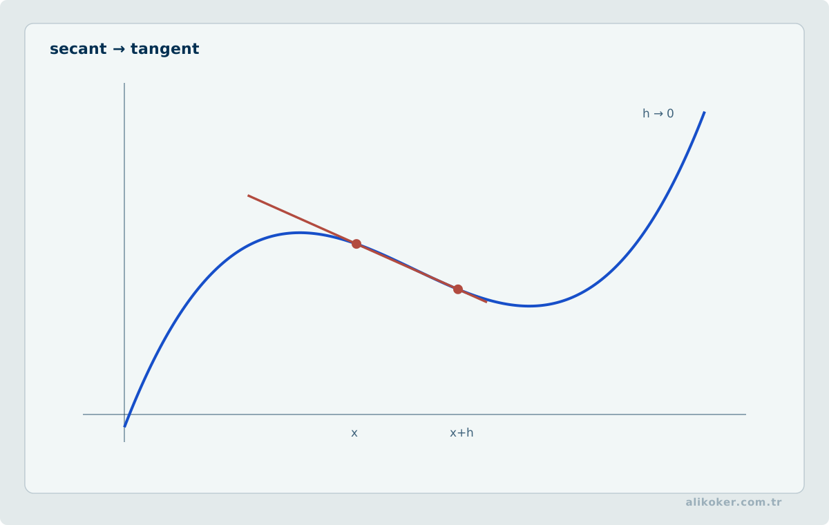
For a graph y=f(x), f'(a) is the slope of the tangent line when the ordinary finite derivative exists:

y-f(a)=f'(a)(x-a).

Physical meaning of the derivative

If s(t) is position, s'(t) is instantaneous velocity and s''(t) acceleration. More generally, derivatives model instantaneous rates of change.

One-sided and infinite derivatives

One-sided derivatives use h→0+ or h→0-. If slopes grow without bound, a vertical-tangent type behavior may be described through an infinite derivative, although this is distinct from having an ordinary finite derivative.

Differential of a function

For a differentiable function,

dy = f'(x) dx.

For a small increment, dy is the linear part of the change in f and provides local approximation.

Basic differentiation rules

(c)'=0
(x^n)'=n x^(n-1)
(f+g)'=f'+g'
(fg)'=f'g+fg'
(f/g)'=(f'g-fg')/g^2.

Derivative of a composite function

The chain rule is

(g∘f)'(x)=g'(f(x)) f'(x).

Derivative of an inverse function

If f is locally invertible and f'(x)≠0, then

(f^-1)'(y)=1/f'(x),  y=f(x).

Derivatives of elementary functions

Standard derivative formulas include exponential, logarithmic, trigonometric, inverse-trigonometric, and hyperbolic functions. Their domain restrictions remain part of the formula.

Logarithmic differentiation

Taking logarithms before differentiating is useful when products, quotients, or variable exponents make direct differentiation cumbersome.

Implicit differentiation

If a relation F(x,y)=0 defines y locally as a function of x, differentiation gives

F_x + F_y y' = 0,

and thus y'=-F_x/F_y when F_y≠0.

Parametric differentiation

For x=x(t), y=y(t),

dy/dx = (dy/dt)/(dx/dt)

when dx/dt≠0.

Higher-order derivatives

Repeated differentiation gives f'', f''', and f^(n). Higher derivatives describe curvature, acceleration, local approximation, and differential-equation structure.

Fermat's theorem and local extrema

At an interior local extremum where f is differentiable,

f'(a)=0.

This is a necessary condition, not a sufficient one.

Rolle's theorem

If f is continuous on [a,b], differentiable on (a,b), and f(a)=f(b), then some c∈(a,b) satisfies

f'(c)=0.

Mean value theorem

If f is continuous on [a,b] and differentiable on (a,b), some c satisfies

f'(c) = [f(b)-f(a)]/(b-a).

Generalized mean value theorem

Cauchy's mean value theorem applies the same idea to two functions and provides a foundation for several limit results.

Taylor formula

Near a,

f(x)=Σ_(k=0)^n f^(k)(a)(x-a)^k/k! + R_n(x).

The remainder controls the error between the function and its polynomial approximation.

Indeterminate forms and L'Hôpital's rule

Under the hypotheses of L'Hôpital's rule, certain 0/0 or ∞/∞ limits can be transformed using derivatives of numerator and denominator. The rule does not apply merely because a quotient looks complicated; the indeterminate form and regularity conditions must first be established.

Constancy and monotonicity tests

On an interval, f'=0 throughout implies constancy under standard differentiability assumptions. The sign of f' determines increasing or decreasing behavior.

Extremum tests

Critical points arise where f'=0 or the derivative is undefined. Sign changes of f' or the second-derivative test can classify suitable critical points.

Convexity, concavity, and inflection points

The sign of f'' provides a local test for convexity/concavity where the second derivative exists. An inflection point requires a change in concavity; f''=0 alone is not sufficient.

Procedure for curve sketching

A systematic sketch can combine domain, symmetry, intercepts, asymptotes, first-derivative monotonicity, extrema, second-derivative concavity, and limiting behavior.

Unit 5: Indefinite Integrals

Antiderivative

F is an antiderivative of f on an interval if

F'(x)=f(x).

Any two antiderivatives on the same interval differ by a constant.

Indefinite integral concept

∫ f(x) dx = F(x)+C.

The constant C represents the family of antiderivatives.

Basic integration formulas

Standard formulas reverse elementary differentiation rules, such as

∫ x^n dx = x^(n+1)/(n+1)+C,  n≠-1
∫ dx/x = ln|x|+C
∫ e^x dx = e^x+C.

Substitution

If u=g(x), then

∫ f(g(x))g'(x) dx = ∫ f(u) du.

Substitution is the inverse pattern of the chain rule.

Integration by parts

From the product rule,

∫ u dv = uv - ∫ v du.

Integration of rational functions

A proper rational function can often be decomposed into partial fractions after factoring the denominator over the relevant field. Improper rational functions are first divided polynomially.

Binomial integrals

Integrals involving powers of x, a+b x^n, or related binomial expressions can sometimes be reduced by substitutions determined by rational-exponent relations. Not every such integral has an elementary antiderivative.

Trigonometric integrals

Powers and products of sine, cosine, tangent, secant, and related functions are handled through identities and substitutions chosen from parity and derivative structure.

Irrational-function integrals

Expressions containing square roots of quadratic forms can often be simplified through trigonometric or algebraic substitutions. The correct substitution depends on the sign pattern of the quadratic expression.

Non-elementary antiderivatives

Some elementary functions do not possess elementary antiderivatives. Examples lead to special functions or numerical integration. The absence of an elementary closed form does not mean the definite integral is meaningless.

Unit 6: Definite Integrals

Partition of an interval

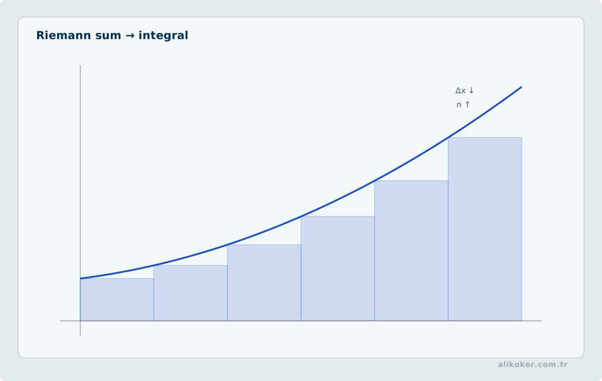
A partition

a=x0<x1<...<xn=b

divides [a,b] into subintervals. Refining the partition is the basis of Riemann integration.

Riemann sum and definite integral

A Riemann sum has the form

Σ f(ξ_i) Δx_i.

If all sufficiently fine partitions lead to one common limit, that limit is the definite integral

∫_a^b f(x) dx.

Lower and upper Darboux sums

Lower sums use infima on each subinterval and upper sums use suprema. A bounded function is Riemann integrable when the gap between upper and lower sums can be made arbitrarily small.

Necessary condition for integrability

A Riemann-integrable function on a closed interval must be bounded. Boundedness alone is not sufficient.

Integrability tests

Every continuous function on [a,b] is Riemann integrable. Bounded functions with only sufficiently mild sets of discontinuities are also integrable under broader criteria.

Properties of the definite integral

Linearity, interval additivity, order comparison, and absolute-value bounds are fundamental properties.

Mean value theorem for integrals

If f is continuous on [a,b], some c∈[a,b] satisfies

∫_a^b f(x)dx = f(c)(b-a).

Fundamental theorem of calculus

If

F(x)=∫_a^x f(t)dt

with continuous f, then F'(x)=f(x). Conversely, if F'=f, then

∫_a^b f(x)dx = F(b)-F(a).

This connects accumulation and differentiation.

Substitution in a definite integral

A change of variables transforms both integrand and limits. Updating the limits avoids mixing variables in the final expression.

Integration by parts in a definite integral

∫_a^b u dv = [uv]_a^b - ∫_a^b v du.

Area of planar regions

The signed integral measures net area relative to the axis. Geometric area requires nonnegative accumulation, or subtraction of lower functions from upper functions over the relevant intervals.

Arc length of a curve

For y=f(x) with appropriate smoothness,

L = ∫_a^b sqrt(1+[f'(x)]^2) dx.

Volume of solids of revolution

Disk/washer and shell methods express volume as definite integrals. The formula depends on the axis of revolution and chosen slicing geometry.

Area of surfaces of revolution

For suitable rotation about an axis, surface area involves the arc-length factor multiplied by the radius to the axis, for example

S = 2π ∫ y sqrt(1+(y')^2) dx

when the geometric assumptions fit.

Center of mass and moment of inertia

Integrals weighted by density give mass, first moments, and moments of inertia. The correct integrand follows from physical geometry and the distance to the selected axis.

Approximate evaluation of definite integrals

When no convenient antiderivative exists, numerical quadrature such as midpoint, trapezoidal, and Simpson-type rules approximates the integral from sampled function values. Their errors depend on step size and smoothness.

Unit 7: Improper Integrals

Types of improper integral

An integral is improper when the interval is unbounded or the integrand becomes unbounded at an endpoint or an interior point. It is defined through limits of proper integrals.

Convergence and divergence

An improper integral converges only if the defining limit exists and is finite. Otherwise it diverges. Splitting at every singular point is necessary.

Fundamental formulas for the first type

For an infinite endpoint,

∫_a^∞ f(x)dx = lim_(b→∞) ∫_a^b f(x)dx.

An integral over (-∞,∞) is defined by separate one-sided improper integrals; cancellation of two divergent sides is not ordinary convergence.

Convergence tests for the first type

Comparison and limit comparison are useful for nonnegative integrands. A standard reference is

∫_1^∞ dx/x^p

which converges exactly when p>1.

Fundamental formulas for the second type

If f is unbounded near a,

∫_a^b f(x)dx = lim_(c→a+) ∫_c^b f(x)dx.

Interior singularities require splitting the interval and checking both sides separately.

Convergence tests for the second type

The comparison model

∫_0^1 dx/x^p

converges exactly when p<1. Comparison and asymptotic equivalence often decide more complicated cases.

General Conceptual Framework

The first course in calculus is organized around local and accumulated change:

Functions
   ↓
Limits
   ↓
Continuity
   ↓
Derivatives
   ↓
Local approximation and qualitative behavior
   ↓
Antiderivatives
   ↓
Definite integrals and accumulation
   ↓
Improper limits and numerical approximation

Limits provide the common language beneath continuity, derivatives, and integrals. Derivatives describe local rate; integrals describe accumulation. The fundamental theorem connects the two operations under appropriate hypotheses.

Conceptual Distinctions

Domain ≠ range. The domain contains admissible inputs; the range contains values actually produced.

Injective ≠ surjective. Injectivity prevents two distinct inputs from sharing one output; surjectivity requires every codomain element to be reached.

Maximum ≠ supremum. A maximum is attained; a supremum need only be the least upper bound.

Function value ≠ limit. f(a) can differ from lim_(x→a)f(x) or even be undefined while the limit exists.

Infinite limit ≠ finite real limit. It describes unbounded behavior rather than convergence to a real number.

Continuity ≠ differentiability. Differentiability implies continuity; continuity does not imply differentiability.

Critical point ≠ extremum. f'=0 or failure of differentiability identifies candidates; additional analysis is needed.

f''(a)=0 ≠ inflection point. Concavity must actually change.

Differential ≠ exact finite change. dy=f'(x)dx is the first-order linear part of the change.

Indefinite integral ≠ definite integral. The first is a family of antiderivatives; the second is a number defined by an accumulation limit.

Signed integral ≠ geometric area. Negative portions subtract in a signed integral.

Improper integral ≠ ordinary integral with infinity as a number. It is defined through a limit.

Numerical quadrature ≠ symbolic antiderivative. Quadrature approximates a definite integral directly from function evaluations.

References

• Ahmet Yesevi Üniversitesi Bilgisayar Mühendisliği Bölümü. Matematik I (TBIL101) ders materyalleri.
• Joel Hass, Christopher Heil, Maurice D. Weir, Przemyslaw Bogacki. Thomas' Calculus, 15th Edition. Pearson, 2022. (Pearson)
• Walter Rudin. Principles of Mathematical Analysis, 3rd Edition. McGraw-Hill, 1976.
• Tom M. Apostol. Calculus, Volume I, 2nd Edition. Wiley, 1967.
• Michael Spivak. Calculus, 4th Edition. Publish or Perish, 2008.
• Richard L. Burden, J. Douglas Faires, Annette M. Burden. Numerical Analysis, 10th Edition. Cengage, 2016.