Discrete Mathematics: Sets, Logic, Relations and Graphs

Discrete Mathematics follows the mathematical language underlying algorithms: sets, logic, relations, combinatorics, and graphs. The topics remain on one backbone so that notation and definitions can be reused consistently across later algorithmic problems.

The subject matters not because it is an easier alternative to continuous mathematics, but because many objects in computer science are inherently discrete. A state machine, reachability relation, truth table, combinatorial count, or graph path shares the same discipline: define the objects precisely and make every inference traceable to explicit rules.

Unit 1: Introduction to Set Theory

Set concept

A set is a well-defined collection of distinct objects called elements. Membership is written as

x ∈ A
x ∉ A.

A set can be described by listing its elements or by specifying a property that characterizes membership.

Venn diagrams

Venn diagrams represent sets as regions and make operations such as union, intersection, difference, and complement visually explicit. They are useful for reasoning but do not replace formal set definitions.

Finite and infinite sets

A finite set has a finite cardinality. Infinite sets contain no finite list of all elements. Different infinite sets can nevertheless be compared through one-to-one correspondences.

Empty set

The empty set ∅ contains no elements. It is a subset of every set and is not the same object as a set that contains the empty set.

Subset and proper subset

A ⊆ B

means every element of A belongs to B. A proper subset is a subset that is not equal to the containing set.

Equality of sets

Two sets are equal exactly when they contain the same elements:

A = B  ⇔  A ⊆ B and B ⊆ A.

Order and repeated listing do not change a set.

Universal set

The universal set U specifies the reference domain in a particular discussion. Complements are always interpreted relative to this universe.

Union

A ∪ B = {x | x∈A or x∈B}.

Intersection

A ∩ B = {x | x∈A and x∈B}.

Disjoint sets have empty intersection.

Complement and difference

A^c = U \ A
A \ B = {x | x∈A and x∉B}.

Symmetric difference

The symmetric difference contains elements that belong to exactly one of the two sets:

A △ B = (A\B) ∪ (B\A).

Ordered pairs and Cartesian product

An ordered pair (a,b) distinguishes first and second components. The Cartesian product is

A x B = {(a,b) | a∈A, b∈B}.

In general A x B and B x A are not the same set.

Boolean algebra of sets

Set operations obey commutative, associative, distributive, identity, absorption, complement, and De Morgan laws. These laws parallel Boolean logic and digital-circuit algebra.

Number sets

The common hierarchy includes natural numbers, integers, rational numbers, real numbers, and complex numbers. Inclusion relations depend on the chosen convention for natural numbers but the structural containment is otherwise standard.

Intervals

Intervals describe subsets of the real line. Parentheses indicate excluded endpoints and brackets included endpoints, with infinity always written as an open boundary.

Absolute value

|x| = x       if x ≥ 0
|x| = -x      if x < 0.

Geometrically, |x-a| is the distance between x and a on the real line.

Integer part

The floor function ⌊x⌋ is the greatest integer less than or equal to x. It is a step function and must not be confused with ordinary rounding.

Unit 2: Permutations and Combinations

Factorial

For a positive integer n,

n! = n(n-1)...2·1,

with 0! = 1 by convention and combinatorial consistency.

Counting principles

The addition rule handles mutually exclusive alternatives. The multiplication rule handles sequential choices. Many combinatorial formulas are direct consequences of these two principles.

Permutation

When order matters, the number of arrangements of r distinct objects chosen from n is

P(n,r) = n!/(n-r)!.

For all n objects, the count is n!.

Permutations with repetition

If a multiset of n objects contains groups of identical elements with multiplicities n1,...,nk, the number of distinct arrangements is

n!/(n1! n2! ... nk!).

Permutation group

All permutations of n objects form the symmetric group S_n under composition. The identity permutation, inverses, closure, and associativity give the group structure.

Combination

When order does not matter,

C(n,r) = n!/[r!(n-r)!].

Properties of combinations

Important identities include

C(n,r) = C(n,n-r)
C(n,r) + C(n,r-1) = C(n+1,r).

These connect combinations with Pascal's triangle and the binomial theorem.

Combinations with repetition

The number of ways to select r items from n types when repetition is allowed is

C(n+r-1,r).

Unit 3: Propositional Logic

Proposition

A proposition is a declarative statement that has a definite truth value, true or false. Questions, commands, and open expressions containing unspecified variables are not propositions until interpreted appropriately.

Compound proposition and truth table

Logical connectives combine propositions into compound propositions. A truth table lists all possible truth-value assignments and the resulting value of the compound expression.

Negation

If p is a proposition, ¬p reverses its truth value.

Conjunction

p ∧ q

is true only when both propositions are true.

Disjunction

The inclusive OR

p ∨ q

is true when at least one operand is true. Exclusive OR is a different operation and is true when exactly one is true.

Conditional proposition

p → q

is false only when p is true and q is false. It is logically equivalent to

¬p ∨ q.

Converse, inverse, and contrapositive

For p→q:

• converse: q→p,
• inverse: ¬p→¬q,
• contrapositive: ¬q→¬p.

The original conditional is logically equivalent to its contrapositive, not generally to its converse or inverse.

Biconditional

p ↔ q

is true when p and q have the same truth value. It represents two implications together.

Equivalent propositions and standard forms

Two formulas are logically equivalent if they have identical truth values under every assignment. Conjunctive and disjunctive normal forms provide systematic representations built from literals.

Tautology and contradiction

A tautology is true under every truth assignment; a contradiction is false under every assignment. A contingency is true for some assignments and false for others.

Laws of logic

Commutative, associative, distributive, identity, idempotent, absorption, double-negation, and De Morgan laws allow expressions to be transformed without changing their truth functions.

Quine method

The Quine-style tabular approach systematically manipulates truth assignments or implicants to simplify Boolean expressions. In digital-logic applications, systematic minimization reduces redundant terms.

Logical circuits

Boolean expressions map naturally to logic gates. AND, OR, and NOT correspond to fundamental gates, while more complex circuits implement compound propositions. Logical equivalence can therefore be used to simplify circuit structure.

Proof patterns for discrete structures

A discrete-mathematics result is stronger when its proof method matches the structure of the statement.

Direct proof starts from the hypotheses and derives the conclusion. Contrapositive proof establishes not Q -> not P instead of P -> Q. Contradiction assumes the negation of the target and derives an impossibility. Mathematical induction proves a base case and an induction step.

For recursive data structures and loops, induction and invariants are closely related. The induction hypothesis describes what remains true after a smaller recursive call; a loop invariant describes what remains true after another iteration.

A counterexample is equally important: one valid counterexample is sufficient to disprove a universal claim.

Unit 4: Relations

Relation concept

A binary relation from A to B is any subset of the Cartesian product:

R ⊆ A x B.

A relation on A is a subset of A x A.

Forms of representation

Relations can be represented as sets of ordered pairs, tables, directed graphs, or zero-one matrices. Each representation emphasizes different operations.

Inverse relation

The inverse relation reverses every ordered pair:

R^-1 = {(b,a) | (a,b)∈R}.

Reflexive relation

A relation on A is reflexive if

(a,a) ∈ R

for every a∈A.

Symmetric relation

It is symmetric if

(a,b)∈R ⇒ (b,a)∈R.

Antisymmetric relation

It is antisymmetric if

(a,b)∈R and (b,a)∈R ⇒ a=b.

Antisymmetry does not mean "not symmetric"; the two properties address different conditions.

Transitive relation

It is transitive if

(a,b)∈R and (b,c)∈R ⇒ (a,c)∈R.

Equivalence relation

An equivalence relation is reflexive, symmetric, and transitive. It divides a set into disjoint equivalence classes.

Equivalence classes and partitions

For an equivalence relation, the class of a is

[a] = {x∈A | xRa}.

Distinct classes are disjoint, and their union is the entire set. Conversely, every partition defines an equivalence relation.

Order relations

A partial order is reflexive, antisymmetric, and transitive. A total order additionally makes every pair comparable. Hasse diagrams provide a compact representation of finite partially ordered sets by omitting implied transitive edges.

Relation matrix

For a finite relation, a zero-one matrix records whether each ordered pair belongs to the relation. Reflexivity, symmetry, and other properties can often be checked from matrix structure.

Closures

A closure adds the minimum information needed to give a relation a desired property, such as reflexive, symmetric, or transitive closure.

Warshall algorithm

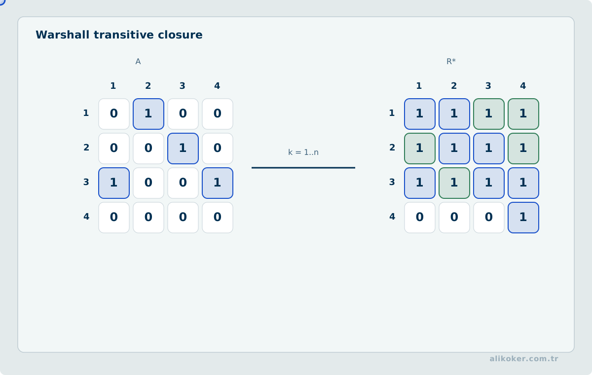
Warshall's algorithm computes transitive closure from an adjacency/relation matrix. At stage k, paths are allowed to use the first k vertices as intermediate points. The Boolean recurrence is

r_ij^(k) = r_ij^(k-1) OR
           (r_ik^(k-1) AND r_kj^(k-1)).

Unit 5: Functions and Operations

Function

A function f:A→B assigns exactly one element of B to every element of A. A function is a special kind of relation with a uniqueness and totality requirement on the domain.

Types of functions

• injective: distinct inputs have distinct outputs;
• surjective: every element of the codomain is reached;
• bijective: both injective and surjective.

A bijection establishes a one-to-one correspondence between the sets.

Inverse function

A function has an inverse function exactly when it is bijective. The inverse reverses input and output roles:

f^-1(f(x)) = x.

Composition

For compatible functions,

(g∘f)(x) = g(f(x)).

Composition is associative but generally not commutative.

Binary operation

A binary operation on A is a function

*: A x A → A.

Closure is therefore built into the definition.

Properties of an operation

Associativity, commutativity, identity elements, and inverses are central properties. Different combinations lead to algebraic structures such as semigroups, monoids, and groups.

Unit 6: Graph Theory

Königsberg bridge problem

Euler's analysis of the Königsberg bridge problem abstracted land regions as vertices and bridges as edges. The problem became a foundational example of graph theory because connectivity, not geometric distance, determined the answer.

Fundamental terminology

A graph consists of vertices and edges. Edges can be undirected or directed, simple or multiple depending on the graph model. Vertex degree counts incident edges in an undirected graph, while directed graphs distinguish indegree and outdegree.

Walk, trail, path, and circuit

A walk is a sequence of adjacent vertices/edges. A trail does not repeat edges; a path usually does not repeat vertices. A closed trail/circuit returns to its starting point. Terminology varies slightly among texts, so the structural restriction should be stated explicitly.

Connectivity and subgraphs

A graph is connected when a path exists between every pair of vertices. A subgraph uses subsets of the original vertices and edges. Connected components are maximal connected subgraphs.

Trees

A tree is a connected undirected graph with no cycles. For a finite tree with n vertices,

number of edges = n - 1.

Between any two vertices of a tree there is a unique simple path.

Directed graphs

Directed edges have orientation. Reachability, paths, and strongly/weakly connected components reflect this direction information.

Structural network analysis: cores, cuts, and directed components

Vertex degree is a local connection count; by itself it does not say whether the vertex lies inside a densely connected interior of the network. k-core decomposition captures this distinction. The k-core is the maximal subgraph in which every remaining vertex has degree at least k within that same subgraph. The largest k for which a vertex remains is its core number.

The basic idea is iterative pruning:

1. remove vertices whose degree is below k
2. update neighbor degrees
3. remove newly under-degree vertices
4. continue until stable

With appropriate degree buckets the full decomposition can be computed in O(V + E). A high core number means that a vertex survives deeper inside a cohesive structural region; it is not, by itself, evidence of leadership, importance, or causal influence. A classical reference is Stephen B. Seidman, Network Structure and Minimum Degree (1983): https://doi.org/10.1016/0378-8733(83)90028-X

Bridges and articulation points also have an algorithmic interpretation. During depth-first search, let disc[v] be the discovery time and low[v] the earliest ancestor reachable from the DFS subtree rooted at v. For a tree edge (u,v),

low[v] > disc[u]

identifies a bridge. For a non-root vertex u, an appropriate child v satisfying

low[v] >= disc[u]

makes u an articulation point. Low-link DFS computes these structures in O(V + E). Robert Tarjan's 1972 paper is a foundational source for linear-time DFS graph algorithms, including strongly and biconnected structures: https://doi.org/10.1137/0201010

For directed graphs, weakly connected components (WCCs) and strongly connected components (SCCs) have different evidence requirements. WCC ignores edge orientation. SCC requires direction-respecting paths between vertices. If an observed relation has unknown direction, silently converting it into two directed edges manufactures structure that was not observed; direction coverage should therefore be treated as part of the interpretation.

Another directed-network measure is PageRank. In a simple form:

PR(v) = (1-d)/N + d * sum(PR(u) / outdeg(u))
                         u -> v

where d is the damping factor and dangling-node mass must be handled explicitly. PageRank depends not only on how many incoming links a vertex has but also on the structural weight of the linking vertices. A high score should still not be translated automatically into social or forensic "importance." The classical large-scale Web treatment is Brin and Page, The Anatomy of a Large-Scale Hypertextual Web Search Engine (1998): https://doi.org/10.1016/S0169-7552(98)00110-X

A classical graph path uses only topology. When edges are events with timestamps, a time-respecting path additionally requires temporal order:

v0 --t1--> v1 --t2--> v2 ... --tk--> vk

t1 <= t2 <= ... <= tk

Applications may also impose a maximum gap between consecutive edges or a maximum total span. A static route can therefore exist while no temporally feasible route exists. This is a useful example of how representation determines which conclusions an algorithm is allowed to make.

Weighted graphs and minimum spanning trees

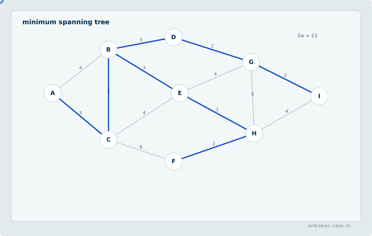
A weighted graph associates costs or lengths with edges. A minimum spanning tree connects all vertices with no cycles and minimum total edge weight. Classical greedy methods include Kruskal and Prim algorithms.

Matrices and graphs

An adjacency matrix records direct edges. Powers of an adjacency matrix encode information about walks of given length, while Boolean matrix operations support reachability computations.

Gantt charts and activity networks

Project activities can be represented by time-oriented Gantt charts or dependency networks. Graph-based scheduling makes precedence relations and critical dependencies explicit; it is conceptually distinct from merely drawing a calendar bar.

Recurrence Relations and Graph Coloring

Many discrete problems have one of two forms: a next value depends on earlier values, or neighboring objects cannot share the same resource. Recurrence relations and graph coloring provide a common mathematical language for these structures.

Recurrence relations

When a sequence term is defined from preceding terms, the result is a recurrence relation:

a_n = 2 a_(n-1) + 1

The recurrence does not identify a unique sequence without an initial condition. With a_0 = 0, it produces:

0, 1, 3, 7, 15, ...

First-order linear recurrences can often be solved algebraically. In divide-and-conquer algorithms, recurrences such as:

T(n) = 2T(n/2) + n

model total work as the problem size shrinks.

The objective is not always a closed form. Monotonicity, upper and lower bounds, and asymptotic growth may be sufficient for algorithmic reasoning.

Graph coloring

In vertex coloring, adjacent vertices are assigned different colors. The minimum number of colors required is the graph's chromatic number.

A --- B
|     |
D --- C

This even cycle can be colored with two colors, whereas an odd cycle cannot.

A graph is bipartite exactly when it is two-colorable; BFS or DFS can test this by assigning alternating colors while traversing edges.

Engineering interpretations

A "color" need not represent a visible color. It can represent a resource or time slot that conflicting items may not share. Examples include:

• exam or job scheduling,
• frequency assignment,
• register allocation,
• resource assignment for conflicting tasks.

The abstraction and the solution method must remain separate. Modeling a problem as a graph exposes its structure; finding an optimal coloring has its own computational cost.

Recurrences and coloring illustrate the same principle: discrete mathematics exposes structural constraints before they are encoded as program logic.

Solving simple recurrence relations

Recurrences express a value through earlier values. They appear in recursive algorithms, counting problems, and dynamic systems.

For T(n)=T(n-1)+c, repeated substitution gives linear growth. For T(n)=2T(n/2)+n, the recursion tree exposes log n levels with approximately n work per level, giving Θ(n log n).

The important step is to state the recurrence from the algorithm before applying a theorem. A wrong recurrence produces a precise answer to the wrong model.

Graph coloring as a resource-allocation model

In graph coloring, adjacent vertices cannot share a color. The abstraction maps naturally to exam scheduling, register allocation, radio-frequency assignment, and other conflict problems.

The chromatic number is a graph property, but finding it exactly is computationally hard in general. Heuristics should therefore be reported as algorithms that produce valid colorings, not as proofs of optimality unless an optimality argument is also available.

Unit 7: Algorithms

Algorithm concept

An algorithm is a finite, unambiguous sequence of effective steps that transforms input into output. Correctness and termination are separate from efficiency.

Pseudocode

Pseudocode expresses control flow independently of a particular programming language. It should be precise enough that the intended algorithm is unambiguous.

Decision structure

Conditional execution selects different steps according to a Boolean condition:

if condition
    action A
else
    action B

Loop structures

Loops repeat computation while a condition holds or over a finite collection. for, while, and repeat-until styles differ in how repetition is controlled.

Subprogram and function

A subprogram encapsulates a reusable computation. Functions additionally emphasize returning a value, although programming-language terminology varies.

Finding the maximum value

A linear scan can find the maximum of n elements by keeping the largest value seen so far. The algorithm requires n-1 comparisons in the ordinary sequential model.

Computer representation of sets

Finite sets over a known universe can be represented by bit vectors. Membership becomes a bit test; union and intersection correspond naturally to bitwise OR and AND.

Computer representation of relations and graphs

Adjacency matrices provide constant-time edge lookup but use quadratic space. Adjacency lists use space proportional to vertices plus edges and are often better for sparse graphs.

Transitive-closure algorithm

Warshall's dynamic-programming recurrence computes reachability for all vertex pairs in O(n^3) time for an n x n relation matrix.

General Conceptual Framework

Discrete mathematics supplies structural language for computer science:

Sets
  ↓
Counting and logic
  ↓
Relations and functions
  ↓
Graphs and algebraic structure
  ↓
Algorithms and representations

Sets define collections and domains. Logic defines valid propositions and transformations. Relations model pairwise structure; functions impose deterministic mapping. Graphs model connectivity and dependency. Algorithms convert these mathematical structures into finite computational procedures.

Conceptual Distinctions

Element ≠ subset. x∈A is membership; B⊆A compares two sets.

Empty set ≠ set containing the empty set. ∅ has zero elements, while {∅} has one element.

Union ≠ intersection. Union uses logical OR; intersection uses logical AND.

Permutation ≠ combination. Permutations distinguish order; combinations do not.

Implication ≠ converse. p→q is equivalent to its contrapositive ¬q→¬p, not generally to q→p.

Tautology ≠ satisfiable formula. A tautology is true under every assignment; a satisfiable formula only needs at least one true assignment.

Symmetric ≠ antisymmetric. Antisymmetry is not the negation of symmetry; a relation can satisfy both in appropriate cases.

Equivalence relation ≠ order relation. Equivalence uses symmetry; partial order uses antisymmetry.

Relation ≠ function. A function must assign exactly one output to each domain element.

Injective ≠ surjective. Injectivity constrains repeated outputs; surjectivity requires the entire codomain to be reached.

Graph ≠ tree. Every tree is a graph, but a tree must be connected and acyclic.

Walk ≠ path. A path imposes stronger nonrepetition conditions than a general walk.

Algorithm ≠ program. An algorithm is an abstract procedure; a program is an implementation in a computational environment.

In discrete mathematics, a strong solution is often determined by representation rather than by a long calculation. Expressing the same problem as a set, relation, proposition, or graph can change both the proof and the algorithm. The core aim is therefore to develop modelling discipline rather than to accumulate formulas.

Invariants and induction as tools for program correctness

Mathematical induction extends naturally to loop invariants. Correctness can be argued through initialization, preservation, and termination.

In binary search, for example, the invariant that a present target remains inside the current search interval exposes off-by-one errors more clearly than random testing alone.

Graph algorithms also rely on invariants: finalized distances in Dijkstra, representative structure in union-find, and indegree conditions in topological sorting are mathematical explanations of why the algorithms work.

Verification with counterexamples and invariants

In discrete mathematics, plausibility is not proof. One counterexample is enough to refute a universal claim, while proving the claim requires a valid argument. The same distinction applies to algorithm correctness.

Small constructed graph cases help expose assumptions: disconnected graphs, cycles, parallel edges, negative weights, and single-node inputs. An algorithm such as Dijkstra can appear to work on some invalid inputs even when its preconditions are violated.

Loop invariants and induction connect program behavior to formal reasoning. Initialization, preservation, and termination provide evidence beyond example outputs.

From Discrete Structures to Search, Planning, and Graph Learning

Discrete mathematics directly supports the symbolic and combinatorial side of AI. Sets, logic, relations, counting, and graphs are natural tools for search, planning, constraint satisfaction, and knowledge representation.

In propositional logic, conclusions follow from explicit premises and inference rules. This differs from statistical learning, where a decision function is estimated from data. Modern systems may combine both: learned perception can produce observations while logical constraints govern admissible actions.

Graph theory creates an even broader bridge. Nodes can represent states, entities, users, or atoms; edges can represent transitions, relations, communication, or chemical bonds. Search operates over a state graph, while graph learning treats the graph itself as data.

A simplified graph-neural-network update is:

h_v^(k+1) = UPDATE(h_v^k, AGGREGATE({h_u^k : u ∈ N(v)}))

The learning mechanism is modern, but neighborhood, path, degree, and connectivity remain graph-theoretic objects.

Combinatorics explains why exhaustive search becomes impossible. The number of permutations of n objects is n!; many scheduling, planning, and feature-subset problems grow too quickly for enumeration. Heuristic search, branch-and-bound, local search, or evolutionary methods become useful because of this combinatorial explosion.

Relations also matter semantically. Equality, similarity, reachability, and ordering do not share the same mathematical properties. A learned similarity score is not necessarily transitive and should not be treated as an equivalence relation without evidence.

Constraint-satisfaction problems provide another direct connection:

X_i ∈ D_i
C_1(X), C_2(X), ...

The objective is to find assignments satisfying the constraints. Scheduling and resource-allocation problems often fit this form. Learning may improve search order, while the meaning of the constraints remains discrete and explicit.

Discrete mathematics is not the sole mathematical foundation of AI. Continuous optimization requires calculus, representation requires linear algebra, and uncertainty requires probability. Its specific contribution is the structure of symbolic inference, graph representation, combinatorial search, and constrained decision problems.

Proof, counterexample, and structure

Checking a statement on several examples is not a proof. One counterexample can refute a universal claim; proving the claim requires definitions, inference rules, or an appropriate proof technique. In particular, P → Q is not equivalent to its converse Q → P. Its contrapositive ¬Q → ¬P, however, is logically equivalent to the original implication.

Induction has two separate obligations: a base case and an induction step. In the step, the goal is to derive P(k+1) from the assumption that P(k) holds; merely computing another example does not establish the implication. Strong induction allows all earlier cases to be used as the induction hypothesis.

For relations, reflexivity, symmetry, antisymmetry, and transitivity are independent properties. An equivalence relation is reflexive, symmetric, and transitive; a partial order is reflexive, antisymmetric, and transitive. The two structures serve different purposes: equivalence relations partition a set into equivalence classes, while partial orders describe comparison structure.

Graph terminology also matters. Paths, trails, cycles, connectivity, and degree are distinct notions. Summing the degrees of all vertices counts each edge twice, so the total is 2|E|. The same handshake lemma explains why the number of odd-degree vertices must be even.

In counting problems, ask first whether order matters, whether repetition is allowed, and whether choices are independent. Those questions usually identify the correct model more reliably than memorising isolated permutation and combination formulas.

From Discrete Mathematics to Formal Languages and Automata

Discrete mathematics is not limited to sets, relations, and graphs. It also provides the mathematical foundation for formal-language theory, which asks which symbol sequences a computational model can recognize and which problems can be solved by which abstract machine. In computer-engineering curricula in Türkiye, this material may follow discrete mathematics directly or appear as a separate course titled Formal Languages and Automata or Automata Theory.

An alphabet is a finite set of symbols. Finite sequences formed from an alphabet are strings, and a set of strings is a language. For example, all binary strings over {0,1} that end in 01 form a language. A formal language does not have to be a programming language; protocol message formats, structured log patterns, and lexical tokens can also be modeled as languages.

Regular languages and finite automata

Regular expressions, regular languages, and finite automata are alternative representations of the same class of expressive power. A deterministic finite automaton (DFA) has exactly one next state for each state and input symbol. A nondeterministic finite automaton (NFA) may permit several possible transitions, but it does not recognize a broader class of languages than a DFA; an equivalent DFA can be constructed by representing sets of NFA states.

input symbols
      ↓
 [initial state]
      ↓
  transitions
      ↓
[accept / reject]

The memory of a finite automaton is limited to its current state. It therefore cannot, in general, recognize structures that require an unbounded stack, such as arbitrarily nested balanced delimiters. This limitation introduces a question that is more fundamental than “which algorithm is faster?”: is the computational model expressive enough for the problem?

Context-free grammars and pushdown automata

Programming-language syntax contains blocks, expressions, and nested structures for which regular languages are often insufficient. A context-free grammar (CFG) uses terminals, nonterminals, productions, and a start symbol to describe richer structures. The natural machine model for this class is the pushdown automaton.

characters
   ↓
lexical analysis            regular language / finite automaton
   ↓
tokens
   ↓
parsing                     CFG / pushdown automaton
   ↓
syntax tree

This distinction connects directly to the compiler pipeline discussed in Programming Languages: lexical analysis and parsing are different computational problems. A string being generated by a grammar also does not imply that a program is semantically valid; type checking, name binding, and runtime behavior belong to later layers.

Turing machines, computability, and decidability

A Turing machine combines finite control with an abstract, unbounded read/write tape. Its purpose is not to imitate a real processor but to define a machine-independent boundary for what it means to be algorithmically computable.

A decision problem requires a yes/no result for every input. If a correct algorithm terminates for every possible input, the problem is decidable. Some problems cannot be solved by any general algorithm for all inputs. The halting problem is important because it demonstrates that no universal, perfect analyzer can determine every relevant property of arbitrary program behavior in advance.

Computability and complexity must remain separate:

computability: Is there an algorithm that solves the problem?
complexity:    If so, how much time or memory does it require?

Automata theory is therefore not merely a historical prerequisite for compiler construction. It supplies a common mathematical vocabulary of state, language, and acceptance used in areas ranging from regular-expression engines and protocol validation to parsing and model checking.

References

• Ahmet Yesevi Üniversitesi Bilgisayar Mühendisliği Bölümü. Ayrık Matematik (TBIL108) ders materyalleri.

• Kenneth H. Rosen. Discrete Mathematics and Its Applications, 8th Edition. McGraw-Hill, 2019.

• Ralph P. Grimaldi. Discrete and Combinatorial Mathematics: An Applied Introduction, 5th Edition. Pearson, 2003.

• Reinhard Diestel. Graph Theory, 5th Edition. Springer, 2017.

• Stuart Russell, P. N. Artificial Intelligence: A Modern Approach, 4th ed. Pearson, 2021.

• Susanna S. Epp. Discrete Mathematics with Applications, 5th Edition. Cengage, 2019.

• Thomas H. Cormen, Charles E. Leiserson, Ronald L. Rivest, Clifford Stein. Introduction to Algorithms, 4th Edition. MIT Press, 2022.