Data Structures and Algorithm Analysis

I kept these data-structures and algorithms notes to study not only what each structure is, but also what each operation costs. This revision retains arrays, linked lists, stacks, queues, trees, hashing and graphs together with algorithm analysis. I distinguish worst-case, average-case and amortized costs where that distinction changes the engineering decision.

Unit 1: Introduction and Fundamental Concepts

Software, programs and hardware

A program is executable logic expressed in some representation; software is broader and includes code, configuration, data, documentation and supporting artifacts. Hardware provides the processor, memory and I/O resources on which software executes.

A data structure sits between the problem's information model and the machine's memory model. Choosing a structure determines not only how values are represented but also which operations are cheap or expensive.

Operating system

The operating system provides abstractions such as processes, virtual memory, files and sockets. Data-structure code ultimately uses resources managed through these abstractions, so memory allocation and I/O costs cannot be ignored when evaluating a real implementation.

Data structure and data model

A data model describes conceptual relationships. A data structure is a concrete organization used to implement operations on data.

For example, a set can be modeled abstractly as an unordered collection of unique elements and implemented with a hash table, balanced tree, bitset or sorted array depending on constraints.

Algorithm

An algorithm is a finite, unambiguous sequence of operations that solves a stated problem. Correctness and complexity are separate questions: an algorithm can be correct but impractically slow or memory-hungry.

Execution speed and memory requirement

Performance must be discussed against input size and workload. One isolated timing number is not an algorithmic complexity result.

Useful questions include:

• how many primitive operations grow with n,
• how much additional memory is required,
• which memory accesses are contiguous or random,
• whether allocation or I/O dominates,
• whether worst-case latency matters more than average throughput.

Processor, machine code and assembly

High-level operations eventually become machine instructions, but source-level operation count does not map one-to-one to CPU cycles. Compilers, caches, branch prediction, vectorization and memory latency all affect actual runtime.

Assembly and machine-code awareness is useful when investigating low-level cost, but asymptotic analysis deliberately abstracts away a particular processor implementation.

Programming languages

The same abstract data structure can have different concrete costs depending on the language/runtime. Manual allocation in C, RAII containers in C++, garbage-collected objects in Java and contiguous numerical arrays in other systems can represent the same logical structure with different memory layouts.

Database and SQL

Database systems implement their own indexing, hashing, trees, sorting and graph-like execution structures. SQL remains declarative, but query performance depends heavily on physical data structures and algorithms chosen by the optimizer.

Divide and conquer

Divide-and-conquer algorithms:

1. divide a problem into smaller subproblems,
2. solve them recursively or iteratively,
3. combine the results.

Merge sort and binary search are classic examples. Recurrence relations describe the cost:

T(n) = a T(n/b) + f(n)

for many divide-and-conquer families.

Benchmarking

A benchmark measures one concrete implementation under one environment. It should include warm-up/runtime effects where relevant, representative data distributions and enough repetitions to distinguish signal from noise.

Benchmark results complement complexity analysis; they do not replace it.

Unit 2: Data Structures and Representation

From raw data to information

Raw values acquire meaning through type, structure and context. A byte sequence can represent text, integers, floating-point numbers, serialized records or instructions depending on interpretation.

Classification

Data structures can be classified in several overlapping ways:

• linear vs non-linear,
• contiguous vs linked,
• static-size vs dynamic,
• ordered vs unordered,
• hierarchical vs network/graph,
• mutable vs immutable.

No classification alone determines performance.

Computer memory

Memory is byte-addressable on common systems, but language objects have alignment, size and lifetime rules. Contiguous structures benefit from spatial locality; pointer-rich structures may incur allocation overhead and cache misses.

Character data

Character representation requires an encoding. ASCII historically maps basic characters to byte values; modern Unicode text may use variable-length encodings such as UTF-8. "One character equals one byte" is not a safe general assumption.

Unsigned and signed integers

An n-bit unsigned integer typically represents:

0 ... 2^n - 1

Two's-complement signed integers represent:

-2^(n-1) ... 2^(n-1)-1

The data structure storing an integer may be simple, but arithmetic overflow behavior depends on the programming language and type.

BCD

Binary-coded decimal stores each decimal digit separately. It uses more bits than pure binary for the same numerical range but preserves decimal digit representation, which can matter in display or decimal-centric systems.

Floating-point values

IEEE 754 binary floating-point represents sign, exponent and significand. Many decimal values are not exactly representable, so comparisons and accumulated numerical error require explicit tolerance/error models where appropriate.

Strings

A string can be represented as:

• a null-terminated character array,
• a length plus contiguous storage,
• immutable shared storage,
• a rope/tree for very large editing workloads,
• language/runtime-specific objects.

Length, encoding and ownership semantics affect complexity.

Arrays

An array stores equal-type elements contiguously:

address(A[i]) = base + i * element_size

Random indexed access is O(1). Inserting/removing in the middle is generally O(n) because elements must move, unless order can be discarded or an indirection scheme is used.

Multidimensional arrays

A multidimensional array maps several indices to one linear storage region according to a layout such as row-major or column-major. Traversal order affects cache locality.

Structures, unions and bit-fields

A structure groups heterogeneous fields and can contain padding for alignment. A union overlays alternatives in one storage region. Bit-fields provide compact implementation-defined packing and are not automatically portable serialized formats.

Unit 3: Data Models

List

A list is an ordered sequence. It can be implemented with arrays, linked nodes, trees or chunked storage depending on operation requirements.

Linked list

A linked list stores links between nodes rather than requiring contiguous element storage. It supports cheap insertion/removal at a known node but has O(n) indexed access and weaker cache locality.

Tree

A tree represents hierarchical parent/child relationships. Many algorithms exploit recursive substructure and logarithmic height when the tree is balanced.

Graph

A graph models general relationships among vertices through edges. Trees are a restricted class of graphs; graph algorithms must account for cycles and multiple paths.

State machine

A state machine is a graph whose nodes are states and edges are transitions conditioned on events/inputs. It is a data/control model used in protocols, parsers and embedded systems.

Relational model

The relational model represents data as relations and uses set-oriented operators. Physical DBMS implementations still rely on arrays, B-trees, hash tables and other structures beneath the logical model.

Network model

Historical network database models represent records and explicit link sets. The concept illustrates the difference between navigation through stored relationships and declarative relational querying.

Unit 4: Algorithmic Program Design

Program design

A reliable design begins from inputs, outputs, invariants and failure conditions. Data structures should be selected after identifying the operations the algorithm must support.

Pseudocode

Pseudocode documents logic without binding it to language syntax. It should be precise about loops, conditions and data updates but need not define machine-level details.

Real code

The implementation adds type rules, memory ownership, error handling, library behavior and performance effects absent from pseudocode. Correct translation therefore requires preserving algorithm invariants, not merely copying control structure.

Flowcharts

Flowcharts can illustrate small decision/loop structures. For large algorithms, pseudocode and data-structure invariants are usually more compact.

Conditional branching and loops

Branching selects between paths. Loops repeat operations while maintaining an invariant. Nested loops do not automatically mean O(n^2); bounds and data dependence must be analyzed.

Quadratic equation roots

For:

a x^2 + b x + c = 0

the discriminant is:

D = b^2 - 4ac

A robust implementation must separately handle a = 0, negative discriminant for real-only output, and numerical precision. The textbook formula demonstrates branching but is also an example where numerical analysis matters.

Arithmetic mean

For n > 0 values:

mean = sum / n

The algorithm is O(n) time and O(1) auxiliary space when streamed. Numeric type and overflow/precision can matter more than asymptotic complexity.

Finding the minimum

A single-pass minimum scan performs n-1 comparisons for non-empty input:

min <- A[0]
for i = 1 .. n-1:
    if A[i] < min:
        min <- A[i]

Time is Theta(n) because every element may have to be inspected.

Unit 5: Time and Space Complexity

Algorithm analysis

Complexity describes resource growth as a function of input size. It intentionally ignores constant machine-specific details when comparing scalability.

Big O

O(g(n)) is an asymptotic upper bound: beyond some point, f(n) is bounded above by a constant multiple of g(n).

Big Omega

Omega(g(n)) is an asymptotic lower bound.

Big Theta

Theta(g(n)) means both upper and lower bounds of the same order.

These notations describe mathematical growth, not automatically worst/best/average cases. One must state which cost function is being bounded.

Common growth classes

Typical orders are:

O(1)
O(log n)
O(n)
O(n log n)
O(n^2)
O(n^3)
O(2^n)
O(n!)

For sufficiently large inputs, growth rate dominates constant-factor differences, although constants and locality remain important in real systems.

Best, average and worst case

Linear search is:

• best case O(1),
• worst case O(n),
• average case O(n) under ordinary position assumptions.

Average-case analysis requires a probability/distribution model; it should not be asserted without one.

Amortized analysis

Amortized analysis distributes occasional expensive operations over a sequence. Dynamic-array append is a classic example: some appends reallocate/copy O(n) elements, but geometric growth yields amortized O(1) append.

Amortized cost is not probabilistic average-case cost.

Space complexity

Space analysis includes auxiliary structures, recursion depth, temporary arrays and metadata. In-place does not always mean O(1) total memory if recursion or runtime stacks grow with input.

Code memory and call stack

Executable code consumes storage largely independently of input size for a fixed program, while recursive call stacks can grow with depth. Quicksort, tree traversal and DFS therefore have stack costs tied to recursion shape.

Benchmark versus analysis

Complexity predicts growth; benchmarking measures one implementation. Cache locality can make an O(n) array scan much faster than an O(n) pointer chase despite the same asymptotic order.

Unit 6: Linked Lists

Singly linked list

A node contains data and a next link:

[data | next] -> [data | next] -> ... -> null

Given a pointer to the insertion location/predecessor, insertion can be O(1). Searching for a value is O(n).

Array versus linked list

Array:

• O(1) indexed access,
• contiguous memory/locality,
• middle insertion/removal usually O(n).

Linked list:

• indexed access O(n),
• insertion/removal at a known node can be O(1),
• per-node allocation and pointer overhead,
• weak spatial locality.

The theoretically cheaper insertion does not make linked lists universally faster.

Doubly linked list

Each node stores previous and next links. Removal of a known node is direct because its predecessor is available, at the cost of another pointer and more link updates.

Circular list

A circular list links the final node back to the first or sentinel. It can simplify repeated round-robin traversal but requires careful termination conditions.

Dynamic allocation and ownership

Each allocated node must have one clear ownership strategy. Failure paths, deletion and list destruction must release every node exactly once.

Insert, search and delete

Head insertion is constant time. Tail insertion is constant time if a tail pointer is maintained, otherwise locating the end is linear.

Deleting by value requires search first (O(n)) unless an external index locates the node. Deleting a known singly linked node usually also needs access to its predecessor.

Sentinel nodes

A sentinel is a non-data boundary node. It reduces special cases for empty/head/tail operations by ensuring links always have a structural endpoint.

Unit 7: Tree Data Model

Trees

A tree is a connected acyclic graph. Rooted trees define parent/child relations, depth and subtrees.

The degree of a node is its number of children in the rooted-tree sense used here; terminology can vary in general graph theory.

Memory representations

Trees can be stored as node objects with child links, arrays for implicit complete trees, or first-child/next-sibling representation for arbitrary numbers of children.

First-child/next-sibling turns an n-ary tree into a binary-link representation:

node -> first child
node -> next sibling

Balanced trees

A balanced search tree keeps height proportional to log n, preventing a sorted/adversarial insertion sequence from degrading ordinary binary search-tree operations to O(n).

AVL tree

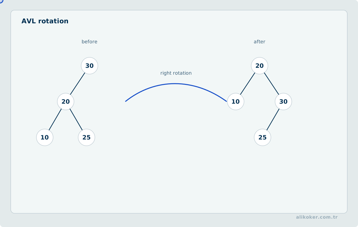
AVL trees maintain a strict balance-factor condition at each node. Rotations restore balance after insertions/deletions. Search, insertion and deletion are O(log n).

Heap

A binary heap is a complete binary tree usually stored in an array. For zero-based indexing:

left(i)  = 2i + 1
right(i) = 2i + 2
parent(i)= floor((i-1)/2)

A min-heap guarantees each parent is no greater than its children; it does not globally sort siblings/subtrees.

Peek is O(1), insert and remove-root are O(log n). Building a heap bottom-up is O(n).

Trie

A trie stores keys by prefixes. Lookup depends on key length rather than directly on number of stored keys:

O(L)

for key length L, subject to child-representation cost. It can consume substantial memory when branching is sparse.

Huffman coding

Huffman coding builds a prefix code by repeatedly combining the two least-frequent symbols/subtrees. With an appropriate priority queue the construction is typically O(k log k) for k symbols.

The result is optimal among prefix codes for the supplied symbol-frequency model in expected code length. It is not a universal compression method by itself; model/header overhead and data distribution matter.

Shannon-Fano

Shannon-Fano recursively partitions symbols into groups with approximately balanced total probability. It is historically important but does not guarantee the same optimal prefix-code result as Huffman's algorithm.

Unit 8: Binary Trees

Binary tree

A binary tree has at most two children per node. A full binary tree commonly means every internal node has exactly two children. A complete binary tree fills all levels except possibly the last, which is filled from left to right. Terminology should be stated because some sources use "full"/"perfect" differently.

Traversals

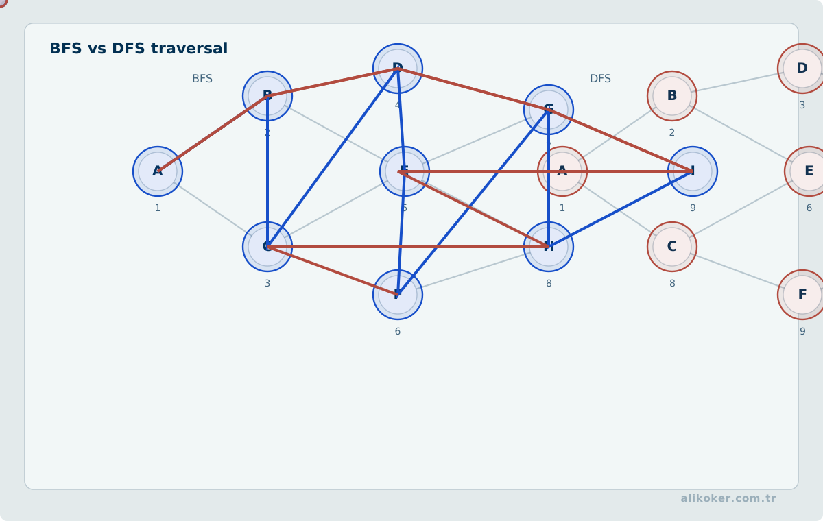
Depth-first traversals are:

preorder:  node, left, right
inorder:   left, node, right
postorder: left, right, node

Breadth-first level-order traversal uses a queue.

For a binary search tree, inorder traversal returns keys in sorted order when the ordering invariant holds.

Expression notations

Expression trees connect traversals to notation:

• inorder -> infix with appropriate parentheses,
• preorder -> prefix,
• postorder -> postfix.

Binary search tree

BST invariant:

keys(left subtree) < key(node) < keys(right subtree)

subject to the chosen duplicate-key policy.

Search, insertion and deletion cost O(h) where h is tree height. A balanced tree has h = O(log n); an unbalanced chain has h = O(n).

Deletion has three structural cases: leaf, one child, two children. For two children, replace using a predecessor/successor strategy and remove that node from its original location.

Unit 9: Stack and Queue

Stack

A stack is LIFO:

push
pop
top/peek

All are O(1) with ordinary array or linked implementations. Uses include call stacks, parsing, expression evaluation, undo and DFS.

An array stack maintains a top index and must handle capacity. A linked stack avoids contiguous resizing but allocates nodes.

Queue

A queue is FIFO:

enqueue -> rear
 dequeue <- front

A naive array queue that shifts elements on every dequeue makes dequeue O(n). A circular buffer uses head/tail indices and achieves O(1) enqueue/dequeue without shifting.

A linked queue maintains front and rear pointers for constant-time operations.

Deque

A double-ended queue permits insertion/removal at both front and rear. It supports algorithms such as sliding-window extrema and can implement both stack- and queue-like behavior.

Priority queue

A priority queue removes the element with highest/lowest priority rather than oldest insertion time. A binary heap is a common implementation with O(log n) insertion/removal and O(1) access to the best element.

Unit 10: Sorting Algorithms

Sorting properties

Sorting arranges records according to a key. Important properties include:

• stable: equal keys preserve relative order,
• in-place: uses only small auxiliary storage under a stated model,
• internal vs external sorting depending on whether data fit in memory.

Insertion sort

Insertion sort maintains a sorted prefix and inserts the next element into it.

• best case O(n) for already sorted data with the usual implementation,
• average/worst O(n^2),
• stable and in-place.

It performs well for small or nearly sorted ranges and is often used inside hybrid sorts.

Selection sort

Selection sort repeatedly selects the minimum remaining element.

• comparisons Theta(n^2) in all ordinary cases,
• few swaps,
• simple but generally not stable in its basic form.

Bubble sort

Bubble sort repeatedly swaps adjacent inverted pairs. Basic complexity is O(n^2); an early-exit flag gives O(n) best case for an already sorted input. It is mostly pedagogical compared with stronger general-purpose algorithms.

Merge sort

Merge sort divides, sorts halves and merges:

T(n) = 2T(n/2) + Theta(n)
     = Theta(n log n)

It is stable with the ordinary merge and works well for linked/external data, but array implementations usually require O(n) auxiliary storage.

Heap sort

Heap sort builds a heap and repeatedly moves the extreme element into final position.

• build heap O(n),
• total O(n log n),
• in-place in an array,
• not stable in its usual form.

Quicksort

Quicksort partitions around a pivot and recursively sorts partitions.

• average/expected O(n log n) with appropriate pivot behavior,
• worst case O(n^2),
• excellent locality and low constants in many array workloads.

Randomized or median-like pivot strategies reduce the likelihood of repeatedly pathological partitions. Recursion depth should be controlled for robustness.

Comparison

No sorting algorithm is universally best. Data size, stability, memory, presortedness, key cost, cache behavior and external-storage constraints determine the choice.

Comparison sorting has a lower bound of Omega(n log n) in the general comparison model. Counting/radix approaches can beat it by exploiting stronger assumptions about keys.

Unit 11: Searching and Hash Tables

Linear search

Linear search scans elements until a match is found. Worst-case time is O(n) and it works without sorted input.

Binary search

Binary search requires ordered random-access data and repeatedly halves the search range:

O(log n)

Boundary arithmetic should avoid overflow, e.g.:

mid = low + (high - low) / 2

The insertion-position and duplicate-key policy must be defined separately from mere existence testing.

Search in BST

BST search follows left/right ordering and costs O(h), which is logarithmic only when height is controlled.

Hash functions and tables

A hash function maps a key to an integer/bucket space. A good non-cryptographic table hash should be fast and distribute expected keys well; it need not provide cryptographic security.

A hash table uses this mapping for average O(1) lookup/insertion under assumptions about load and distribution. Worst-case behavior can be O(n).

Collisions

Different keys can map to the same bucket. Collision handling is therefore required.

Separate chaining stores multiple entries per bucket, commonly in lists or small structures.

Open addressing stores entries in the table itself and probes alternative slots.

Linear, quadratic and double-hash probing

Linear probing has excellent locality but primary clustering. Quadratic probing changes probe spacing to reduce clustering. Double hashing derives a probe step from another hash function and can spread probes more broadly.

Probe sequences must be compatible with table size so an available slot can be reached.

Load factor and rehashing

Load factor:

alpha = number_of_entries / number_of_buckets

Strongly affects expected probe/chain cost. A table resizes and rehashes when its policy threshold is reached. Resize is expensive but amortized over many insertions.

Unit 12: Graphs

Graph model

A graph is:

G = (V, E)

with vertices V and edges E.

Graphs may be undirected, directed, weighted or unweighted. Degree counts incident edges in undirected graphs; directed graphs distinguish in-degree and out-degree.

A path is a sequence of adjacent vertices/edges. A cycle returns to its starting vertex under the graph's direction rules.

Representations

Adjacency matrix uses O(V^2) memory and gives constant-time edge-existence checks.

Adjacency list uses roughly O(V + E) memory and is efficient for sparse graphs and neighbor traversal.

Edge list stores edge tuples and is convenient for algorithms such as Kruskal.

An incidence matrix represents vertex-edge incidence and is distinct from an adjacency matrix.

DFS

Depth-first search explores as far as possible before backtracking. With adjacency lists:

O(V + E)

It can be implemented recursively or with an explicit stack. Uses include cycle analysis, connected components and topological-order construction.

BFS

Breadth-first search explores vertices by increasing unweighted distance from a source using a queue. With adjacency lists it is also O(V + E) and finds shortest path lengths in unweighted graphs.

Greedy approach

A greedy algorithm makes locally optimal choices without revisiting them. Greedy correctness depends on problem structure; the strategy is not valid merely because each step looks best locally.

Dijkstra

Dijkstra's algorithm computes shortest paths from one source when edge weights are non-negative. With a binary heap and adjacency lists, a common complexity is:

O((V + E) log V)

often simplified to O(E log V) for connected sparse graphs. Negative edge weights invalidate Dijkstra's correctness assumptions.

Minimum spanning tree

For a connected undirected weighted graph, an MST connects all vertices with minimum total edge weight and no cycles.

Kruskal sorts edges by weight and adds an edge when it joins different components. Disjoint Set Union efficiently tracks components.

With sorting:

O(E log E)

is typical.

Prim grows one tree by repeatedly adding the cheapest edge crossing from the built set to an outside vertex. With a heap it has complexity similar to Dijkstra's form on sparse adjacency lists.

Disjoint Set Union

DSU supports:

find(x)
union(a, b)

With path compression and union by rank/size, amortized operation cost is nearly constant, formally involving the inverse Ackermann function.

Graph coloring

Graph coloring assigns colors so adjacent vertices differ. General minimum vertex coloring is computationally hard; greedy coloring is fast but does not guarantee the minimum number of colors.

Topological sorting

A topological order exists only for a directed acyclic graph. Kahn's algorithm repeatedly removes zero-in-degree vertices; DFS can also construct a reverse finishing order. Detecting that not all vertices can be processed reveals a cycle.

Using Data Structures Together

Real systems rarely use one isolated structure. A graph algorithm may use adjacency lists, a hash map for identifiers, a heap for priorities, a queue for work and a DSU for connectivity. The design question is therefore not "which data structure is fastest" but which combination supports the required operations under the actual data scale and latency/memory constraints.

The core relationship is:

problem operations
      ↓
data model
      ↓
data structure
      ↓
algorithm
      ↓
time + memory + locality cost

Complexity analysis defines scalability. Concrete memory layout and implementation determine whether that theoretical advantage survives on real hardware.

References

- Mark Allen Weiss. Data Structures and Algorithm Analysis in C++. Pearson, 2012.
- Robert Sedgewick; Kevin Wayne. Algorithms. Addison-Wesley, 2011.
- Stuart Russell, P. N. Artificial Intelligence: A Modern Approach, 4th ed. Pearson, 2021.
- Thomas H. Cormen; Charles E. Leiserson; Ronald L. Rivest; Clifford Stein. Introduction to Algorithms. MIT Press, 2009.